Rows built on a quantitative basis, are called variational.
The distribution series consist of options(characteristic values) and frequencies(number of groups). Frequencies expressed as relative values (fractions, percentages) are called frequencies. The sum of all frequencies is called the volume of the distribution series.
By type, the distribution series are divided into discrete(constructed based on discontinuous values of the characteristic) and interval(based on continuous values of the characteristic).
Variation series represents two columns (or rows); one of which contains individual values a varying characteristic, called variants and denoted by X; and in the other - absolute numbers showing how many times (how often) each option occurs. The indicators in the second column are called frequencies and are conventionally denoted by f. Let us note once again that in the second column relative indicators can be used, characterizing the share of the frequency of individual options in the total sum of frequencies. These relative indicators are called frequencies and are conventionally denoted by ω The sum of all frequencies in this case is equal to one. However, frequencies can also be expressed as percentages, and then the sum of all frequencies gives 100%.
If options variation series expressed in the form of discrete quantities, then such a variation series is called discrete.
For continuous characteristics, variation series are constructed as interval, that is, the values of the attribute in them are expressed “from... to...”. In this case, the minimum values of the characteristic in such an interval are called the lower limit of the interval, and the maximum - the upper limit.
Interval variation series are also constructed for discrete characteristics that vary over a large range. Interval series can be with equal And unequal at intervals.
Let's consider how the value of equal intervals is determined. Let us introduce the following notation:
i– interval size;
- the maximum value of the characteristic for population units;
– the minimum value of the characteristic for population units;
n – number of allocated groups.
, if n is known.
If the number of groups to be identified is difficult to determine in advance, then to calculate the optimal interval size with a sufficient population size, the formula proposed by Sturgess in 1926 can be recommended:
n = 1+ 3.322 log N, where N is the number of units in the aggregate.
The size of unequal intervals is determined in each individual case, taking into account the characteristics of the object of study.
Statistical sample distribution call a list of options and their corresponding frequencies (or relative frequencies).
The statistical distribution of the sample can be specified in the form of a table, in the first column of which the options are located, and in the second - the frequencies corresponding to these options ni, or relative frequencies Pi .
Statistical distribution of the sample
Interval series are variation series in which the values of the characteristics underlying their formation are expressed within certain limits (intervals). Frequencies in this case refer not to individual values of the attribute, but to the entire interval.
Interval distribution series are constructed based on continuous quantitative characteristics, as well as on discrete characteristics that vary within significant limits.
An interval series can be represented by the statistical distribution of a sample indicating the intervals and their corresponding frequencies. In this case, the sum of the frequencies of the variants falling within this interval is taken as the frequency of the interval.
When grouping by quantitative continuous characteristics, determining the size of the interval is important.
In addition to the sample mean and sample variance, other characteristics of the variation series are also used.
Fashion The variant that has the highest frequency is called.
- Introductory lesson for free;
- A large number of experienced teachers (native and Russian-speaking);
- Courses are NOT for a specific period (month, six months, year), but for a specific number of lessons (5, 10, 20, 50);
- More than 10,000 satisfied customers.
- The cost of one lesson with a Russian-speaking teacher is from 600 rubles, with a native speaker - from 1500 rubles
The concept of a variation series. The first step in systematizing statistical observation materials is to count the number of units that have a particular characteristic. By arranging the units in ascending or descending order of their quantitative characteristic and counting the number of units with a specific value of the characteristic, we obtain a variation series. A variation series characterizes the distribution of units of a certain statistical population according to some quantitative characteristic.
The variation series consists of two columns, the left column contains the values of the varying characteristic, called variants and denoted (x), and the right column contains absolute numbers showing how many times each variant occurs. The indicators in this column are called frequencies and are designated (f).
The variation series can be schematically presented in the form of Table 5.1:
Table 5.1
Type of variation series
|
Options (x) |
Frequencies (f) |
In the right column, relative indicators can also be used, characterizing the share of the frequency of individual options in the total sum of frequencies. These relative indicators are called frequencies and are conventionally denoted by , i.e. . The sum of all frequencies is equal to one. Frequencies can also be expressed as percentages, and then their sum will be equal to 100%.
Varying signs may be different character. Variants of some characteristics are expressed in integers, for example, the number of rooms in an apartment, the number of books published, etc. These signs are called discontinuous or discrete. Variants of other characteristics can take on any values within certain limits, such as, for example, the implementation of planned tasks, wage etc. These signs are called continuous.
Discrete variation series. If the variants of a variation series are expressed in the form of discrete quantities, then such a variation series is called discrete, it appearance presented in table. 5.2:
Table 5.2
Distribution of students according to exam grades
|
Ratings (x) |
Number of students (f) |
In % of total () |
The nature of the distribution in discrete series is depicted graphically in the form of a distribution polygon, Fig. 5.1.

Rice. 5.1. Distribution of students according to grades obtained on the exam.
Interval variation series. For continuous characteristics, variation series are constructed as interval ones, i.e. the values of the characteristic in them are expressed in the form of intervals “from and to”. In this case, the minimum value of the characteristic in such an interval is called the lower limit of the interval, and the maximum is called the upper limit of the interval.
Interval variation series are constructed both for discontinuous characteristics (discrete) and for those varying over a large range. Interval rows can be with equal or unequal intervals. In economic practice, most unequal intervals are used, progressively increasing or decreasing. This need arises especially in cases where the fluctuation of a characteristic occurs unevenly and within large limits.
Let's consider the type of interval series with equal intervals, table. 5.3:
Table 5.3
Distribution of workers by production
|
Output, t.r. (X) |
Number of workers (f) |
Cumulative frequency (f´) |
The interval distribution series is graphically depicted in the form of a histogram, Fig. 5.2.

Fig.5.2. Distribution of workers by production
Accumulated (cumulative) frequency. In practice, there is a need to transform distribution series into cumulative series, built according to accumulated frequencies. With their help, you can determine structural averages that facilitate the analysis of distribution series data.
Cumulative frequencies are determined by sequentially adding to the frequencies (or frequencies) of the first group these indicators of subsequent groups of the distribution series. Cumulates and ogives are used to illustrate distribution series. To construct them, the values of the discrete characteristic (or the ends of the intervals) are marked on the abscissa axis, and the cumulative totals of frequencies (cumulates) are marked on the ordinate axis, Fig. 5.3.

Rice. 5.3. Cumulative distribution of workers by production
If the scales of frequencies and options are reversed, i.e. the abscissa axis reflects the accumulated frequencies, and the ordinate axis shows the values of the variants, then the curve characterizing the change in frequencies from group to group will be called the distribution ogive, Fig. 5.4.

Rice. 5.4. Ogiva of distribution of workers by production
Variation series with equal intervals provide one of the most important requirements for statistical distribution series, ensuring their comparability in time and space.
Distribution density. However, the frequencies of individual unequal intervals in the named series are not directly comparable. In such cases, to ensure the necessary comparability, the distribution density is calculated, i.e. determine how many units in each group are per unit of interval value.
When constructing a graph of the distribution of a variation series with unequal intervals, the height of the rectangles is determined in proportion not to the frequencies, but to the density indicators of the distribution of the values of the characteristic being studied in the corresponding intervals.
Drawing up a variation series and its graphic image is the first step in processing the initial data and the first stage in the analysis of the population being studied. Next step in the analysis of variation series is the determination of the main general indicators, called the characteristics of the series. These characteristics should give an idea of the average value of the characteristic among population units.
average value. The average value is a generalized characteristic of the characteristic being studied in the population under study, reflecting its typical level per unit of the population under specific conditions of place and time.
The average value is always named and has the same dimension as the characteristic of individual units of the population.
Before calculating average values, it is necessary to group the units of the population under study, identifying qualitatively homogeneous groups.
The average calculated for the population as a whole is called the overall average, and for each group - group averages.
There are two types of averages: power (arithmetic mean, harmonic mean, geometric mean, quadratic mean); structural (mode, median, quartiles, deciles).
The choice of average for calculation depends on the purpose.
Types of power averages and methods for their calculation. In the practice of statistical processing of collected material, various problems arise, the solution of which requires different averages.
Mathematical statistics derives various averages from power average formulas:
where is the average value; x – individual options (feature values); z – exponent (with z = 1 – arithmetic mean, z = 0 geometric mean, z = - 1 – harmonic mean, z = 2 – square mean).
However, the question of what type of average should be applied in each individual case is resolved through a specific analysis of the population being studied.
The most common type of average in statistics is arithmetic mean. It is calculated in cases where the volume of the averaged characteristic is formed as the sum of its values for individual units of the statistical population being studied.
Depending on the nature of the source data, the arithmetic mean is determined in various ways:
If the data is ungrouped, then the calculation is carried out using the simple average formula
Calculation of the arithmetic mean in a discrete series occurs according to formula 3.4.
Calculation of the arithmetic mean in an interval series. In an interval variation series, where the value of a characteristic in each group is conventionally taken to be the middle of the interval, the arithmetic mean may differ from the mean calculated from ungrouped data. Moreover, the larger the interval in the groups, the greater the possible deviations of the average calculated from grouped data from the average calculated from ungrouped data.
When calculating the average over an interval variation series, to perform the necessary calculations, one moves from the intervals to their midpoints. And then the average is calculated using the weighted arithmetic average formula.
Properties of the arithmetic mean. The arithmetic mean has some properties that make it possible to simplify calculations; let’s consider them.
1. The arithmetic mean of constant numbers is equal to this constant number.
If x = a. Then  .
.
2. If the weights of all options are changed proportionally, i.e. increase or decrease by the same number of times, then the arithmetic mean of the new series will not change.
If all weights f are reduced by k times, then  .
.
3. The sum of positive and negative deviations of individual options from the average, multiplied by the weights, is equal to zero, i.e. ![]()
If, then. From here.
If all options are reduced or increased by any number, then the arithmetic mean of the new series will decrease or increase by the same amount.
Let's reduce all options x on a, i.e. x´ = x– a.
Then 
The arithmetic mean of the original series can be obtained by adding to the reduced mean the number previously subtracted from the variants a, i.e. .
5. If all options are reduced or increased in k times, then the arithmetic mean of the new series will decrease or increase by the same amount, i.e. V k once.
Let it be then  .
.
Hence, i.e. to obtain the average of the original series, the arithmetic average of the new series (with reduced variants) must be increased by k once.
Harmonic mean. The harmonic mean is the reciprocal of the arithmetic mean. It is used when statistical information does not contain frequencies for individual variants of the population, but is presented as their product (M = xf). The harmonic mean will be calculated using formula 3.5
|
|

The practical application of the harmonic mean is to calculate some indices, in particular, the price index.
Geometric mean. When using geometric mean, individual values of a characteristic are, as a rule, relative values of dynamics, constructed in the form of chain values, as a ratio to the previous level of each level in a series of dynamics. The average thus characterizes the average growth rate.
The geometric mean value is also used to determine the equidistant value from the maximum and minimum values of the characteristic. For example, an insurance company enters into contracts for the provision of auto insurance services. Depending on the specific insured event insurance payment can range from $10,000 to $100,000 per year. The average amount of insurance payments will be USD.
The geometric mean is a quantity used as the average of ratios or in distribution series presented in the form of a geometric progression when z = 0. This mean is convenient to use when attention is paid not to absolute differences, but to the ratios of two numbers.
The formulas for calculation are as follows
where are the variants of the characteristic being averaged; – product of options; f– frequency of options.
The geometric mean is used in calculations of average annual growth rates.
Mean square. The mean square formula is used to measure the degree of fluctuation of individual values of a characteristic around the arithmetic mean in the distribution series. Thus, when calculating variation indicators, the average is calculated from the squared deviations of individual values of a characteristic from the arithmetic mean.
The root mean square value is calculated using the formula
|
|

In economic research, the modified mean square is widely used in calculating indicators of variation of a characteristic, such as dispersion and standard deviation.
Majority rule. There is the following relationship between power averages - the larger the exponent, the greater the value of the average, Table 5.4:
Table 5.4
Relationship between averages
|
z value |
||||
|
Relationship between averages |
This relationship is called the majorancy rule.
Structural averages. To characterize the structure of the population, special indicators are used, which can be called structural averages. These indicators include mode, median, quartiles and deciles.
Fashion. Mode (Mo) is the most frequently occurring value of a characteristic among population units. The mode is the value of the attribute that corresponds to the maximum point of the theoretical distribution curve.
Fashion is widely used in commercial practice when studying consumer demand (when determining the sizes of clothes and shoes that are in wide demand), and recording prices. There may be several mods in total.
Calculation of mode in a discrete series. In a discrete series, mode is the variant with the highest frequency. Let's consider finding a mode in a discrete series.
Calculation of mode in an interval series. In an interval variation series, the mode is approximately considered to be the central variant of the modal interval, i.e. the interval that has the highest frequency (frequency). Within the interval, you need to find the value of the attribute that is the mode. For an interval series, the mode will be determined by the formula
|
|

Where - bottom line modal interval; – the value of the modal interval; – frequency corresponding to the modal interval; – frequency preceding the modal interval; – frequency of the interval following the modal one.
Median. Median () is the value of the attribute of the middle unit of the ranked series. A ranked series is a series in which the characteristic values are written in ascending or descending order. Or the median is a value that divides the number of an ordered variation series into two equal parts: one part has a value of the varying characteristic that is less than the average option, and the other has a value that is greater.
To find the median, first determine its ordinal number. To do this, if the number of units is odd, one is added to the sum of all frequencies and everything is divided by two. With an even number of units, the median is found as the value of the attribute of a unit, the serial number of which is determined by the total sum of frequencies divided by two. Knowing the serial number of the median, it is easy to find its value using the accumulated frequencies.
Calculation of the median in a discrete series. According to the sample survey, data on the distribution of families by number of children was obtained, table. 5.5. To determine the median, we first determine its ordinal number
= ![]()
Then we will construct a series of accumulated frequencies (, using the serial number and the accumulated frequency we will find the median. The accumulated frequency of 33 shows that in 33 families the number of children does not exceed 1 child, but since the number of the median is 50, the median will be in the range from 34 to 55 families.
Table 5.5
Distribution of the number of families based on the number of children
|
Number of children in the family |
Number of families, – the value of the median interval; All considered forms of power averages have an important property (unlike structural averages) - the formula for determining the average includes all values of the series, i.e. the size of the average is influenced by the value of each option. On the one hand, this is a very positive property because in this case, the effect of all causes affecting all units of the population under study is taken into account. On the other hand, even one observation included in the source data by chance can significantly distort the idea of the level of development of the trait being studied in the population under consideration (especially in short series). Quartiles and deciles. By analogy with finding the median in variation series, you can find the value of a characteristic for any unit of the ranked series. So, in particular, you can find the value of the attribute for units dividing a series into 4 equal parts, into 10, etc. Quartiles. The options that divide the ranked series into four equal parts are called quartiles. In this case, they distinguish: the lower (or first) quartile (Q1) - the value of the attribute for a unit of the ranked series, dividing the population in the ratio of ¼ to ¾ and the upper (or third) quartile (Q3) - the value of the attribute for the unit of the ranked series, dividing the population in the ratio ¾ to ¼. The second quartile is the median Q2 = Me. The lower and upper quartiles in an interval series are calculated using a formula similar to the median. where is the lower limit of the interval containing the lower and upper quartiles, respectively; – accumulated frequency of the interval preceding the interval containing the lower or upper quartile; – frequencies of quartile intervals (lower and upper) The intervals containing Q1 and Q3 are determined by the accumulated frequencies (or frequencies). Deciles. In addition to quartiles, deciles are calculated - options that divide the ranked series into 10 equal parts. They are designated by D, the first decile D1 divides the series in the ratio of 1/10 and 9/10, the second D2 - 2/10 and 8/10, etc. They are calculated according to the same scheme as the median and quartiles. Both the median, quartiles, and deciles belong to the so-called ordinal statistics, which is understood as an option that occupies a certain ordinal place in the ranked series. |
Depending on the characteristic underlying the formation of the distribution series, there are attributive and variational distribution series.
The presence of a common characteristic is the basis for the formation of a statistical population, which represents the results of describing or measuring the general characteristics of the objects of study.
The subject of study in statistics is changing (varying) characteristics or statistical characteristics.
Types of statistical characteristics.
Distribution series are called attributive built according to quality criteria. Attributive– this is a sign that has a name (for example, profession: seamstress, teacher, etc.).
The distribution series is usually presented in the form of tables. In table 2.8 shows the attribute distribution series.
Table 2.8 - Distribution of types of legal assistance provided by lawyers to citizens of one of the regions of the Russian Federation.
Variation series are distribution series, built on a quantitative basis. Any variation series consists of two elements: options and frequencies.
Variants are considered to be the individual values of a characteristic that it takes in a variation series.
Frequencies are the numbers of individual variants or each group of a variation series, i.e. These are numbers showing how often certain options occur in a distribution series. The sum of all frequencies determines the size of the entire population, its volume.
Frequencies are frequencies expressed as fractions of a unit or as a percentage of the total. Accordingly, the sum of the frequencies is equal to 1 or 100%. The variation series allows one to estimate the form of the distribution law based on actual data.
Depending on the nature of the variation of the trait, there are discrete and interval variation series.
An example of a discrete variation series is given in table. 2.9.
Table 2.9 - Distribution of families by the number of occupied rooms in individual apartments in 1989 in the Russian Federation.
Variation series
A certain quantitative characteristic is studied in the general population. A sample of volume is randomly extracted from it n, that is, the number of sample elements is equal to n. At the first stage of statistical processing, ranging samples, i.e. number ordering x 1 , x 2 , …, x n Ascending. Each observed value x i called option. Frequency m i is the number of observations of the value x i in the sample. Relative frequency (frequency) w i is the frequency ratio m i to sample size n: .When studying variation series, the concepts of accumulated frequency and accumulated frequency are also used. Let x some number. Then the number of options , whose values are less x, is called the accumulated frequency: for x i
A characteristic is called discretely variable if its individual values (variants) differ from each other by a certain finite value (usually an integer). The variation series of such a characteristic is called a discrete variation series.
Table 1. General view of a discrete variation frequency series
| Characteristic values | x i | x 1 | x 2 | … | x n |
| Frequencies | m i | m 1 | m 2 | … | m n |
A characteristic is called continuously varying if its values differ from each other by an arbitrarily small amount, i.e. a sign can take any value in a certain interval. A continuous variation series for such a characteristic is called interval.
Table 2. General view of the interval variation series of frequencies
Table 3. Graphic images of the variation series
| Row | Polygon or histogram | Empirical distribution function | |
| Discrete | 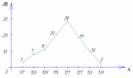 |  | 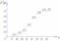 |
| Interval |  |  |  |
For graphical representation of variation series, the polygon, histogram, cumulative curve and empirical distribution function are most often used.
In table 2.3 (Grouping of the Russian population by average per capita income in April 1994) is presented interval variation series.
It is convenient to analyze distribution series using a graphical image, which allows one to judge the shape of the distribution. A visual representation of the nature of changes in the frequencies of the variation series is given by polygon and histogram.
The polygon is used when depicting discrete variation series.
Let us, for example, graphically depict the distribution of housing stock by type of apartment (Table 2.10).
Table 2.10 - Distribution of the housing stock of the urban area by type of apartment (conditional figures).

Rice. Housing distribution area
Not only the frequency values, but also the frequencies of the variation series can be plotted on the ordinate axes.
The histogram is used to depict an interval variation series. When constructing a histogram, the values of the intervals are plotted on the abscissa axis, and the frequencies are depicted by rectangles built on the corresponding intervals. The height of the columns in the case of equal intervals should be proportional to the frequencies. A histogram is a graph in which a series is depicted as bars adjacent to each other.
Let us graphically depict the interval distribution series given in table. 2.11.
Table 2.11 - Distribution of families by size of living space per person (conditional figures).
| N p/p | Groups of families by size of living space per person | Number of families with a given size of living space | Cumulative number of families |
| 1 | 3 – 5 | 10 | 10 |
| 2 | 5 – 7 | 20 | 30 |
| 3 | 7 – 9 | 40 | 70 |
| 4 | 9 – 11 | 30 | 100 |
| 5 | 11 – 13 | 15 | 115 |
| TOTAL | 115 | ---- | |

Rice. 2.2. Histogram of the distribution of families by the size of living space per person
Using the data of the accumulated series (Table 2.11), we construct cumulate distribution.

Rice. 2.3. Cumulative distribution of families by size of living space per person
The representation of a variation series in the form of a cumulate is especially effective for variation series whose frequencies are expressed as fractions or percentages of the sum of the series frequencies.
If we change the axes when graphically depicting a variation series in the form of cumulates, then we get ogiva. In Fig. 2.4 shows an ogive constructed on the basis of the data in Table. 2.11.
A histogram can be converted into a distribution polygon by finding the midpoints of the sides of the rectangles and then connecting these points with straight lines. The resulting distribution polygon is shown in Fig. 2.2 with a dotted line.
When constructing a histogram of the distribution of a variation series with unequal intervals, it is not the frequencies that are plotted along the ordinate axis, but the density of the distribution of the characteristic in the corresponding intervals.
The distribution density is the frequency calculated per unit interval width, i.e. how many units in each group are per unit of interval value. An example of calculating the distribution density is presented in table. 2.12.
Table 2.12 - Distribution of enterprises by number of employees (conditional figures)
| N p/p | Groups of enterprises by number of employees, people. | Number of enterprises | Interval size, people. | Distribution density |
| A | 1 | 2 | 3=1/2 | |
| 1 | Up to 20 | 15 | 20 | 0,75 |
| 2 | 20 – 80 | 27 | 60 | 0,25 |
| 3 | 80 – 150 | 35 | 70 | 0,5 |
| 4 | 150 – 300 | 60 | 150 | 0,4 |
| 5 | 300 – 500 | 10 | 200 | 0,05 |
| TOTAL | 147 | ---- | ---- |
Can also be used to graphically represent variation series cumulative curve. Using a cumulate (sum curve), a series of accumulated frequencies is depicted. Cumulative frequencies are determined by sequentially summing frequencies across groups and show how many units in the population have attribute values no greater than the value under consideration.

Rice. 2.4. Ogive of distribution of families by the size of living space per person
When constructing the cumulates of an interval variation series, variants of the series are plotted along the abscissa axis, and accumulated frequencies are plotted along the ordinate axis.
Continuous variation series
Continuous variation series - a series constructed on the basis of a quantitative statistical characteristic. Example. The average duration of illness of convicts (days per person) in the autumn-winter period this year was:| 7,0 | 6,0 | 5,9 | 9,4 | 6,5 | 7,3 | 7,6 | 9,3 | 5,8 | 7,2 |
| 7,1 | 8,3 | 7,5 | 6,8 | 7,1 | 9,2 | 6,1 | 8,5 | 7,4 | 7,8 |
| 10,2 | 9,4 | 8,8 | 8,3 | 7,9 | 9,2 | 8,9 | 9,0 | 8,7 | 8,5 |
An example of solving a test on mathematical statistics
Problem 1
Initial data : students of a certain group consisting of 30 people passed an exam in the “Informatics” course. The grades received by students form the following series of numbers:
I. Let's create a variation series
|
m x |
w x |
m x nak |
w x nak |
|
|
Total: |
II. Graphic representation of statistical information.

III. Numerical characteristics of the sample.
1. Arithmetic mean
2. Geometric mean
3. Fashion 
4. Median
222222333333333 | 3 34444444445555

5. Sample variance

7. Coefficient of variation

8. Asymmetry
9. Asymmetry coefficient

10. Excess
11. Kurtosis coefficient

Problem 2
Initial data : Students of a certain group wrote a final test. The group consists of 30 people. The points scored by students form the following series of numbers
Solution
I. Since the characteristic takes on many different values, we will construct an interval variation series for it. To do this, first set the interval value h. Let's use Stanger's formula
Let's create an interval scale. In this case, we will take as the upper limit of the first interval the value determined by the formula:
We determine the upper boundaries of subsequent intervals using the following recurrent formula:
 , Then
We finish constructing the interval scale, since the upper limit of the next interval has become greater than or equal to the maximum sample value  .
.
|
|
|
|
|
|


II. Graphic display of interval variation series


III. Numerical characteristics of the sample
To determine the numerical characteristics of the sample, we will compile an auxiliary table
|
|
|
|
|
|
|
|
Sum: |


1. Arithmetic mean

2. Geometric mean
3. Fashion 
4. Median
10 11 12 12 13 13 13 13 14 14 14 14 15 15 15 |15 15 15 16 16 16 16 16 17 17 18 19 19 20 20

5. Sample variance

6. Sample standard deviation

7. Coefficient of variation

8. Asymmetry

9. Asymmetry coefficient

10. Excess

11. Kurtosis coefficient

Problem 3
Condition : the ammeter scale division value is 0.1 A. Readings are rounded to the nearest whole division. Find the probability that during the reading an error will be made that exceeds 0.02 A.
Solution.
The rounding error of the sample can be considered as a random variable X, which is distributed evenly in the interval between two adjacent integer divisions. Uniform distribution density
 ,
,
Where  - length of the interval containing possible values X; outside this interval
  In this problem, the length of the interval containing possible values is X, is equal to 0.1, so

The reading error will exceed 0.02 if it is in the interval (0.02; 0.08). Then
Answer: R=0,6
Problem 4
Initial data: mathematical expectation and standard deviation of a normally distributed characteristic X respectively equal to 10 and 2. Find the probability that as a result of the test X will take the value contained in the interval (12, 14).
Solution.
Let's use the formula

And theoretical frequencies 


For X its mathematical expectation is M(X) and variance D(X). Solution. Let's find the distribution function F(x) of the random variable... sampling error). Let's compose variational row Interval width will be: For each value row Let's calculate how many...
Solution: separable equation
SolutionIn the form of To find the quotient solutions inhomogeneous equation let's make up system Let's solve the resulting system... ; +47; +61; +10; -8. Build interval variational row. Give statistical estimates of the average value...
Solution: Let's calculate chain and basic absolute increases, growth rates, growth rates. We summarize the obtained values in Table 1
SolutionVolume of production. Solution: Arithmetic mean of interval variational row is calculated as follows: for... Marginal sampling error with probability 0.954 (t=2) will be: Δ w = t*μ = 2*0.0146 = 0.02927 Let’s define the boundaries...
Solution. Sign
SolutionAbout whose work experience and made up sample. The sample average work experience... of these employees and made up sample. The average duration for the sample... 1.16, significance level α = 0.05. Solution. Variational row of this sample looks like: 0.71 ...
Working curriculum in biology for grades 10-11 Compiled by: Polikarpova S. V.
Working curriculumThe simplest crossing schemes" 5 L.r. " Solution elementary genetic problems" 6 L.r. " Solution elementary genetic problems" 7 L.r. "..., 110, 115, 112, 110. Compose variational row, draw variational curve, find the average value of the characteristic...
A group of numbers united by some characteristic is called as a whole.
As noted above, primary statistical sports material is a group of disparate numbers that do not give the coach an idea of the essence of the phenomenon or process. The challenge is to turn this collection into a system and use its indicators to obtain the required information.
The compilation of a variation series is precisely the formation of a certain mathematical
Example 2. 34 skiers recorded the following heart rate recovery time after completing the distance (in seconds):
81; 78: 84; 90; 78; 74; 84; 85; 81; 84: 79; 84; 74; 84; 84;
85; 81; 84; 78: 81; 74; 84; 81; 84; 85; 81; 78; 81; 81; 84;
As you can see, this group of numbers does not carry any information.
To compile a variation series, we first perform the operation ranking - arranging numbers in ascending or descending order. For example, in ascending order the ranking results in the following;
78; 78; 78; 78; 78; 78;
81; 81; 81; 81; 81; 81; 81; 81; 81;
84; 84; 84; 84; 84; 84; 84; 84; 84; 84; 84;
In descending order, the ranking results in this group of numbers:
84; 84; 84; 84; 84; 84; 84; 84: 84: 84; 84;
81; 81; 81; 81; 8!; 81: 81; 81; 81;
78; 78; 78; 78; 78; 78;
After the ranking, the irrational form of writing this group of numbers becomes obvious - the same numbers are repeated many times. Therefore, the natural idea arises to transform the record in such a way as to indicate which number is repeated how many times. For example, given the ranking in ascending order:
Here on the left is a number indicating the recovery time of the athlete’s pulse, on the right is the number of repetitions of this reading in a given group of 34 athletes.
In accordance with the above concepts about mathematical symbols, we will denote the considered group of measurements by some letter, for example x. Considering the increasing order of numbers in this group: x 1 -74 s; x 2 - 78 s; x 3 - 81 s; x 4 - 84 s; x 5 - 85 s; x 6 - x n - 90 s, each number considered can be denoted by the symbol X i.
Let us denote the number of repetitions of the considered measurements by the letter n. Then:
n 1 =4; n 2 =6; n 3 =9; n 4 =11; n 5 =3;n 6 =n n =1, and each number of repetitions can be denoted as n i.
The total number of measurements taken, as follows from the example condition, is 34. This means that the sum of all n is equal to 34. Or in symbolic expression:
Let's denote this amount with one letter - n. Then the initial data of the example under consideration can be written in this form (Table 1).
The resulting group of numbers is a transformed series of chaotically scattered readings obtained by the trainer at the beginning of work.
Table 1
| x i | n i |
| n=34 |
Such a group represents a specific system, the parameters of which characterize the measurements taken. The numbers representing the results of measurements (x i) are called options; n i - the number of their repetitions - are called frequencies; n - sum of all frequencies - yes volume of the population.
The entire resulting system is called variation series. Sometimes these series are called empirical or statistical.
It is easy to see that a special case of a variational series is possible when all frequencies are equal to one n i ==1, that is, each measurement in a given group of numbers occurs only once.
The resulting variation series, like any other, can be represented graphically. To plot a graph of the resulting series, it is necessary first of all to agree on the scale on the horizontal and vertical axis.
In this problem, we will plot the values of the pulse recovery time (x 1) on the horizontal axis in such a way that a unit of length, chosen arbitrarily, corresponds to the value of one second. We will begin to postpone these values from 70 seconds, conditionally retreating from the intersection of the two axes 0.
On the vertical axis we plot the frequency values of our series (n i), taking the scale: a unit of length is equal to a unit of frequency.
Having thus prepared the conditions for constructing a graph, we begin to work with the resulting variation series.
We plot the first pair of numbers x 1 =74, n 1 =4 on the graph like this: on the x axis; find x 1 =74 and restore the perpendicular from this point, on the n axis we find n 1 = 4 and draw a horizontal line from it until it intersects with the previously restored perpendicular. Both lines—vertical and horizontal—are auxiliary lines and therefore are drawn dotted on the drawing. The point of their intersection represents, on the scale of this graph, the ratio X 1 =74 and n 1 =4.
All other points on the graph are plotted in the same way. Then they are connected by straight segments. In order for the graph to have a closed appearance, we connect the extreme points with segments to adjacent points of the horizontal axis.
The resulting figure is a graph of our variation series (Fig. 1).
It is absolutely clear that each variation series is represented by its own graph.

Rice. 1. Graphic representation of the variation series.
In Fig. 1 visible:
1) of all those examined, the largest group consisted of athletes whose heart rate recovery time was 84 s;
2) for many this time is 81 s;
3) the smallest group consisted of athletes with a short pulse recovery time - 74 s and a long one - 90 s.
Thus, after completing a series of tests, you should rank the numbers obtained and compile a variation series, which is a certain mathematical system. For clarity, the variation series can be illustrated with a graph.
The above variation series is also called discrete next to it - one in which each option is expressed by one number.
Let us give a few more examples of compiling variation series.
Example 3. 12 shooters, performing a prone exercise of 10 shots, showed the following results (in points):
94; 91; 96; 94; 94; 92; 91; 92; 91; 95; 94; 94.
To form a variation series, we will rank these numbers;
94; 94; 94; 94; 94;
After ranking, we compile a variation series (Table 3).