An ordered pair (X , Y) of random variables X and Y is called a two-dimensional random variable, or a random vector of a two-dimensional space. A two-dimensional random variable (X,Y) is also called a system of random variables X and Y. The set of all possible values of a discrete random variable with their probabilities is called the distribution law of this random variable. A discrete two-dimensional random variable (X, Y) is considered given if its distribution law is known:
P(X=x i , Y=y j) = p ij , i=1,2...,n, j=1,2...,m
Service assignment. Using the service, according to a given distribution law, you can find:
- distribution series X and Y, mathematical expectation M[X], M[Y], variance D[X], D[Y];
- covariance cov(x,y), correlation coefficient r x,y , conditional distribution series X, conditional expectation M;
Instruction. Specify the dimension of the probability distribution matrix (number of rows and columns) and its form. The resulting solution is saved in a Word file.
Example #1. A two-dimensional discrete random variable has a distribution table:
| Y/X | 1 | 2 | 3 | 4 |
| 10 | 0 | 0,11 | 0,12 | 0,03 |
| 20 | 0 | 0,13 | 0,09 | 0,02 |
| 30 | 0,02 | 0,11 | 0,08 | 0,01 |
| 40 | 0,03 | 0,11 | 0,05 | q |
Decision. We find the value q from the condition Σp ij = 1
Σp ij = 0.02 + 0.03 + 0.11 + … + 0.03 + 0.02 + 0.01 + q = 1
0.91+q = 1. Whence q = 0.09
Using the formula ∑P(x i,y j) = p i(j=1..n), find the distribution series X.
M[y] = 1*0.05 + 2*0.46 + 3*0.34 + 4*0.15 = 2.59
Dispersion D[Y] = 1 2 *0.05 + 2 2 *0.46 + 3 2 *0.34 + 4 2 *0.15 - 2.59 2 = 0.64
Standard deviationσ(y) = sqrt(D[Y]) = sqrt(0.64) = 0.801
covariance cov(X,Y) = M - M[X] M[Y] = 2 10 0.11 + 3 10 0.12 + 4 10 0.03 + 2 20 0.13 + 3 20 0.09 + 4 20 0.02 + 1 30 0.02 + 2 30 0.11 + 3 30 0.08 + 4 30 0.01 + 1 40 0.03 + 2 40 0.11 + 3 40 0.05 + 4 40 0.09 - 25.2 2.59 = -0.068
Correlation coefficient rxy = cov(x,y)/σ(x)&sigma(y) = -0.068/(11.531*0.801) = -0.00736
Example 2 . The data of statistical processing of information regarding two indicators X and Y are reflected in the correlation table. Required:
- write distribution series for X and Y and calculate sample means and sample standard deviations for them;
- write conditional distribution series Y/x and calculate conditional averages Y/x;
- graphically depict the dependence of the conditional averages Y/x on the values of X;
- calculate the sample correlation coefficient Y on X;
- write a sample direct regression equation;
- represent geometrically the data of the correlation table and build a regression line.
The set of all possible values of a discrete random variable with their probabilities is called the distribution law of this random variable.
A discrete two-dimensional random variable (X,Y) is considered given if its distribution law is known:
P(X=x i , Y=y j) = p ij , i=1,2...,n, j=1,2...,m
| X/Y | 20 | 30 | 40 | 50 | 60 |
| 11 | 2 | 0 | 0 | 0 | 0 |
| 16 | 4 | 6 | 0 | 0 | 0 |
| 21 | 0 | 3 | 6 | 2 | 0 |
| 26 | 0 | 0 | 45 | 8 | 4 |
| 31 | 0 | 0 | 4 | 6 | 7 |
| 36 | 0 | 0 | 0 | 0 | 3 |
1. Dependence of random variables X and Y.
Find the distribution series X and Y.
Using the formula ∑P(x i,y j) = p i(j=1..n), find the distribution series X. Mathematical expectation M[Y].
M[y] = (20*6 + 30*9 + 40*55 + 50*16 + 60*14)/100 = 42.3
Dispersion D[Y].
D[Y] = (20 2 *6 + 30 2 *9 + 40 2 *55 + 50 2 *16 + 60 2 *14)/100 - 42.3 2 = 99.71
Standard deviation σ(y).
Since, P(X=11,Y=20) = 2≠2 6, then the random variables X and Y dependent.
2. Conditional distribution law X.
Conditional distribution law X(Y=20).
P(X=11/Y=20) = 2/6 = 0.33
P(X=16/Y=20) = 4/6 = 0.67
P(X=21/Y=20) = 0/6 = 0
P(X=26/Y=20) = 0/6 = 0
P(X=31/Y=20) = 0/6 = 0
P(X=36/Y=20) = 0/6 = 0
Conditional expectation M = 11*0.33 + 16*0.67 + 21*0 + 26*0 + 31*0 + 36*0 = 14.33
Conditional variance D = 11 2 *0.33 + 16 2 *0.67 + 21 2 *0 + 26 2 *0 + 31 2 *0 + 36 2 *0 - 14.33 2 = 5.56
Conditional distribution law X(Y=30).
P(X=11/Y=30) = 0/9 = 0
P(X=16/Y=30) = 6/9 = 0.67
P(X=21/Y=30) = 3/9 = 0.33
P(X=26/Y=30) = 0/9 = 0
P(X=31/Y=30) = 0/9 = 0
P(X=36/Y=30) = 0/9 = 0
Conditional expectation M = 11*0 + 16*0.67 + 21*0.33 + 26*0 + 31*0 + 36*0 = 17.67
Conditional variance D = 11 2 *0 + 16 2 *0.67 + 21 2 *0.33 + 26 2 *0 + 31 2 *0 + 36 2 *0 - 17.67 2 = 5.56
Conditional distribution law X(Y=40).
P(X=11/Y=40) = 0/55 = 0
P(X=16/Y=40) = 0/55 = 0
P(X=21/Y=40) = 6/55 = 0.11
P(X=26/Y=40) = 45/55 = 0.82
P(X=31/Y=40) = 4/55 = 0.0727
P(X=36/Y=40) = 0/55 = 0
Conditional expectation M = 11*0 + 16*0 + 21*0.11 + 26*0.82 + 31*0.0727 + 36*0 = 25.82
Conditional variance D = 11 2 *0 + 16 2 *0 + 21 2 *0.11 + 26 2 *0.82 + 31 2 *0.0727 + 36 2 *0 - 25.82 2 = 4.51
Conditional distribution law X(Y=50).
P(X=11/Y=50) = 0/16 = 0
P(X=16/Y=50) = 0/16 = 0
P(X=21/Y=50) = 2/16 = 0.13
P(X=26/Y=50) = 8/16 = 0.5
P(X=31/Y=50) = 6/16 = 0.38
P(X=36/Y=50) = 0/16 = 0
Conditional expectation M = 11*0 + 16*0 + 21*0.13 + 26*0.5 + 31*0.38 + 36*0 = 27.25
Conditional variance D = 11 2 *0 + 16 2 *0 + 21 2 *0.13 + 26 2 *0.5 + 31 2 *0.38 + 36 2 *0 - 27.25 2 = 10.94
Conditional distribution law X(Y=60).
P(X=11/Y=60) = 0/14 = 0
P(X=16/Y=60) = 0/14 = 0
P(X=21/Y=60) = 0/14 = 0
P(X=26/Y=60) = 4/14 = 0.29
P(X=31/Y=60) = 7/14 = 0.5
P(X=36/Y=60) = 3/14 = 0.21
Conditional expectation M = 11*0 + 16*0 + 21*0 + 26*0.29 + 31*0.5 + 36*0.21 = 30.64
Conditional variance D = 11 2 *0 + 16 2 *0 + 21 2 *0 + 26 2 *0.29 + 31 2 *0.5 + 36 2 *0.21 - 30.64 2 = 12.37
3. Conditional distribution law Y.
Conditional distribution law Y(X=11).
P(Y=20/X=11) = 2/2 = 1
P(Y=30/X=11) = 0/2 = 0
P(Y=40/X=11) = 0/2 = 0
P(Y=50/X=11) = 0/2 = 0
P(Y=60/X=11) = 0/2 = 0
Conditional expectation M = 20*1 + 30*0 + 40*0 + 50*0 + 60*0 = 20
Conditional variance D = 20 2 *1 + 30 2 *0 + 40 2 *0 + 50 2 *0 + 60 2 *0 - 20 2 = 0
Conditional distribution law Y(X=16).
P(Y=20/X=16) = 4/10 = 0.4
P(Y=30/X=16) = 6/10 = 0.6
P(Y=40/X=16) = 0/10 = 0
P(Y=50/X=16) = 0/10 = 0
P(Y=60/X=16) = 0/10 = 0
Conditional expectation M = 20*0.4 + 30*0.6 + 40*0 + 50*0 + 60*0 = 26
Conditional variance D = 20 2 *0.4 + 30 2 *0.6 + 40 2 *0 + 50 2 *0 + 60 2 *0 - 26 2 = 24
Conditional distribution law Y(X=21).
P(Y=20/X=21) = 0/11 = 0
P(Y=30/X=21) = 3/11 = 0.27
P(Y=40/X=21) = 6/11 = 0.55
P(Y=50/X=21) = 2/11 = 0.18
P(Y=60/X=21) = 0/11 = 0
Conditional expectation M = 20*0 + 30*0.27 + 40*0.55 + 50*0.18 + 60*0 = 39.09
Conditional variance D = 20 2 *0 + 30 2 *0.27 + 40 2 *0.55 + 50 2 *0.18 + 60 2 *0 - 39.09 2 = 44.63
Conditional distribution law Y(X=26).
P(Y=20/X=26) = 0/57 = 0
P(Y=30/X=26) = 0/57 = 0
P(Y=40/X=26) = 45/57 = 0.79
P(Y=50/X=26) = 8/57 = 0.14
P(Y=60/X=26) = 4/57 = 0.0702
Conditional expectation M = 20*0 + 30*0 + 40*0.79 + 50*0.14 + 60*0.0702 = 42.81
Conditional variance D = 20 2 *0 + 30 2 *0 + 40 2 *0.79 + 50 2 *0.14 + 60 2 *0.0702 - 42.81 2 = 34.23
Conditional distribution law Y(X=31).
P(Y=20/X=31) = 0/17 = 0
P(Y=30/X=31) = 0/17 = 0
P(Y=40/X=31) = 4/17 = 0.24
P(Y=50/X=31) = 6/17 = 0.35
P(Y=60/X=31) = 7/17 = 0.41
Conditional expectation M = 20*0 + 30*0 + 40*0.24 + 50*0.35 + 60*0.41 = 51.76
Conditional variance D = 20 2 *0 + 30 2 *0 + 40 2 *0.24 + 50 2 *0.35 + 60 2 *0.41 - 51.76 2 = 61.59
Conditional distribution law Y(X=36).
P(Y=20/X=36) = 0/3 = 0
P(Y=30/X=36) = 0/3 = 0
P(Y=40/X=36) = 0/3 = 0
P(Y=50/X=36) = 0/3 = 0
P(Y=60/X=36) = 3/3 = 1
Conditional expectation M = 20*0 + 30*0 + 40*0 + 50*0 + 60*1 = 60
Conditional variance D = 20 2 *0 + 30 2 *0 + 40 2 *0 + 50 2 *0 + 60 2 *1 - 60 2 = 0
covariance.
cov(X,Y) = M - M[X] M[Y]
cov(X,Y) = (20 11 2 + 20 16 4 + 30 16 6 + 30 21 3 + 40 21 6 + 50 21 2 + 40 26 45 + 50 26 8 + 60 26 4 + 40 31 4 + 50 31 6 + 60 31 7 + 60 36 3)/100 - 25.3 42.3 = 38.11
If the random variables are independent, then their covariance is zero. In our case cov(X,Y) ≠ 0.
Correlation coefficient.
The linear regression equation from y to x is:
The linear regression equation from x to y is:
Find the necessary numerical characteristics.
Sample means:
x = (20(2 + 4) + 30(6 + 3) + 40(6 + 45 + 4) + 50(2 + 8 + 6) + 60(4 + 7 + 3))/100 = 42.3
y = (20(2 + 4) + 30(6 + 3) + 40(6 + 45 + 4) + 50(2 + 8 + 6) + 60(4 + 7 + 3))/100 = 25.3
dispersions:
σ 2 x = (20 2 (2 + 4) + 30 2 (6 + 3) + 40 2 (6 + 45 + 4) + 50 2 (2 + 8 + 6) + 60 2 (4 + 7 + 3) )/100 - 42.3 2 = 99.71
σ 2 y = (11 2 (2) + 16 2 (4 + 6) + 21 2 (3 + 6 + 2) + 26 2 (45 + 8 + 4) + 31 2 (4 + 6 + 7) + 36 2 (3))/100 - 25.3 2 = 24.01
Where do we get the standard deviations:
σ x = 9.99 and σ y = 4.9
and covariance:
Cov(x,y) = (20 11 2 + 20 16 4 + 30 16 6 + 30 21 3 + 40 21 6 + 50 21 2 + 40 26 45 + 50 26 8 + 60 26 4 + 40 31 4 + 50 31 6 + 60 31 7 + 60 36 3)/100 - 42.3 25.3 = 38.11
Let's define the correlation coefficient:
Let's write down the equations of the regression lines y(x):
and calculating, we get:
yx = 0.38x + 9.14
Let's write down the equations of regression lines x(y):
and calculating, we get:
x y = 1.59 y + 2.15
If we build the points defined by the table and the regression lines, we will see that both lines pass through the point with coordinates (42.3; 25.3) and the points are located close to the regression lines.
Significance of the correlation coefficient.

According to Student's table with significance level α=0.05 and degrees of freedom k=100-m-1 = 98 we find t crit:
t crit (n-m-1;α/2) = (98;0.025) = 1.984
where m = 1 is the number of explanatory variables.
If t obs > t is critical, then the obtained value of the correlation coefficient is recognized as significant (the null hypothesis asserting that the correlation coefficient is equal to zero is rejected).
Since t obl > t crit, we reject the hypothesis that the correlation coefficient is equal to 0. In other words, the correlation coefficient is statistically significant.
Exercise. The number of hits of pairs of values of random variables X and Y in the corresponding intervals are given in the table. From these data, find the sample correlation coefficient and the sample equations of the straight regression lines Y on X and X on Y .
Decision
Example. The probability distribution of a two-dimensional random variable (X, Y) is given by a table. Find the laws of distribution of the component quantities X, Y and the correlation coefficient p(X, Y).
Download Solution
Exercise. A two-dimensional discrete value (X, Y) is given by a distribution law. Find the distribution laws of the X and Y components, covariance and correlation coefficient.
Let a two-dimensional random variable $(X,Y)$ be given.
Definition 1
The distribution law of a two-dimensional random variable $(X,Y)$ is the set of possible pairs of numbers $(x_i,\ y_j)$ (where $x_i \epsilon X,\ y_j \epsilon Y$) and their probabilities $p_(ij)$ .
Most often, the distribution law of a two-dimensional random variable is written in the form of a table (Table 1).
Figure 1. Law of distribution of a two-dimensional random variable.
Let's remember now theorem on the addition of probabilities of independent events.
Theorem 1
The probability of the sum of a finite number of independent events $(\ A)_1$, $(\ A)_2$, ... ,$\ (\ A)_n$ is calculated by the formula:
Using this formula, one can obtain distribution laws for each component of a two-dimensional random variable, that is:
From here it will follow that the sum of all probabilities of a two-dimensional system has the following form:
Let us consider in detail (step by step) the problem associated with the concept of the distribution law of a two-dimensional random variable.
Example 1
The distribution law of a two-dimensional random variable is given by the following table:
Figure 2.
Find the laws of distribution of random variables $X,\ Y$, $X+Y$ and check in each case that the total sum of probabilities is equal to one.
- Let us first find the distribution of the random variable $X$. The random variable $X$ can take the values $x_1=2,$ $x_2=3$, $x_3=5$. To find the distribution, we will use Theorem 1.
Let us first find the sum of probabilities $x_1$ as follows:

Figure 3
Similarly, we find $P\left(x_2\right)$ and $P\left(x_3\right)$:
\ \
Figure 4
- Let us now find the distribution of the random variable $Y$. The random variable $Y$ can take the values $x_1=1,$ $x_2=3$, $x_3=4$. To find the distribution, we will use Theorem 1.
Let us first find the sum of probabilities $y_1$ as follows:

Figure 5
Similarly, we find $P\left(y_2\right)$ and $P\left(y_3\right)$:
\ \
Hence, the law of distribution of the quantity $X$ has the following form:
Figure 6
Let's check the fulfillment of the equality of the total sum of probabilities:
- It remains to find the law of distribution of the random variable $X+Y$.
Let's designate it for convenience through $Z$: $Z=X+Y$.
First, let's find what values this quantity can take. To do this, we will pairwise add the values of $X$ and $Y$. We get the following values: 3, 4, 6, 5, 6, 8, 6, 7, 9. Now, discarding the matched values, we get that the random variable $X+Y$ can take the values $z_1=3,\ z_2=4 ,\ z_3=5,\ z_4=6,\ z_5=7,\ z_6=8,\ z_7=9.\ $
First, let's find $P(z_1)$. Since the value of $z_1$ is single, it is found as follows:
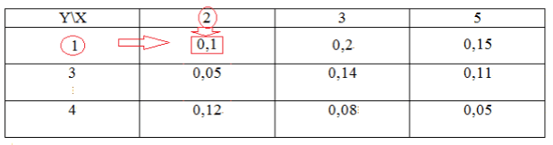
Figure 7
All probabilities are found similarly, except for $P(z_4)$:
Let us now find $P(z_4)$ as follows:
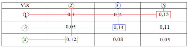
Figure 8
Hence, the distribution law for $Z$ has the following form:
Figure 9
Let's check the fulfillment of the equality of the total sum of probabilities:
Definition. If two random variables are given on the same space of elementary events X and Y, then they say that it is given two-dimensional random variable (X,Y) .
Example. The machine stamps steel tiles. Length controlled X and width Y. − two-dimensional SW.
SW X and Y have their own distribution functions and other characteristics.
Definition. The distribution function of a two-dimensional random variable (X, Y) is called a function.
Definition. The distribution law of a discrete two-dimensional random variable (X, Y) called a table
| … | ||||
| … | ||||
For a two-dimensional discrete SW .
Properties :
2) if , then ; if , then ;
4) − distribution function X;
− distribution function Y.
Probability of hitting the values of the two-dimensional SW in the rectangle:
Definition. 2D random variable (X,Y) called continuous if its distribution function is continuous on and has everywhere (with the possible exception of a finite number of curves) a continuous mixed partial derivative of the 2nd order .
Definition. The density of the joint probability distribution of the two-dimensional continuous SW is called a function.
Then obviously .
Example 1 The two-dimensional continuous SW is given by the distribution function
Then the distribution density has the form
Example 2 The two-dimensional continuous SW is given by the distribution density
Let's find its distribution function:
Properties :
3) for any area.
Let the joint distribution density be known. Then the distribution density of each of the components of the two-dimensional SW is found as follows:
Example 2 (continued).
The distribution densities of the two-dimensional SW components are called by some authors marginal probability distribution densities .
Conditional laws of distribution of components of the system of discrete RV.
Conditional probability , where .
Conditional distribution law of the component X at :
| X | … | |||
| R | … |
Similarly for , where .
Let's make a conditional distribution law X at Y= 2.
Then the conditional distribution law
| X | -1 | ||
| R |
Definition. The conditional distribution density of the X component at a given value Y=y called .
Similarly: .
Definition. conditional mathematical waiting for discrete SW Y at is called , where − see above.
Hence, .
For continuous SW Y .
Obviously is a function of the argument X. This function is called regression function Y on X .
Similarly defined x-on-y regression function : .
Theorem 5. (On the distribution function of independent RVs)
SW X and Y
Consequence. Continuous SW X and Y are independent if and only if .
In example 1 with . Therefore, SW X and Y independent.
Numerical characteristics of the components of a two-dimensional random variable
For discrete CB:
For continuous SW: .
Dispersion and standard deviation for all SW are determined by the same formulas known to us:
Definition. The point is called scattering center two-dimensional SW.
Definition. Covariance (correlation moment) NE is called
For discrete SW: .
For continuous SW: .
Formula for calculation: .
For independent CBs.
The inconvenience of the characteristic is its dimension (the square of the unit of measurement of the components). The following quantity is free from this shortcoming.
Definition. Correlation coefficient SW X and Y called
For independent CBs.
For any pair of SW . It is known that if and only if , where .
Definition. SW X and Y called uncorrelated , if .
Relationship between correlation and dependence of SW:
− if CB X and Y correlated, i.e. , then they are dependent; the reverse is not true;
− if CB X and Y independent, then ; the opposite is not true.
Remark 1. If SW X and Y distributed according to the normal law and , then they are independent.
Remark 2. Practical value as a measure of dependence is justified only when the joint distribution of the pair is normal or approximately normal. For arbitrary SW X and Y you can come to an erroneous conclusion, i.e. may be even when X and Y associated with a strict functional relationship.
Remark 3. In mathematical statistics, a correlation is a probabilistic (statistical) dependence between quantities that, generally speaking, does not have a strictly functional character. Correlation dependence occurs when one of the quantities depends not only on the given second, but also on a number of random factors, or when among the conditions on which one or the other quantity depends, there are conditions common to both of them.
Example 4 For SW X and Y from example 3 find .
Decision.
Example 5 The joint distribution density of the two-dimensional SW is given.
An ordered pair (X , Y) of random variables X and Y is called a two-dimensional random variable, or a random vector of a two-dimensional space. A two-dimensional random variable (X,Y) is also called a system of random variables X and Y. The set of all possible values of a discrete random variable with their probabilities is called the distribution law of this random variable. A discrete two-dimensional random variable (X, Y) is considered given if its distribution law is known:
P(X=x i , Y=y j) = p ij , i=1,2...,n, j=1,2...,m
Service assignment. Using the service, according to a given distribution law, you can find:
- distribution series X and Y, mathematical expectation M[X], M[Y], variance D[X], D[Y];
- covariance cov(x,y), correlation coefficient r x,y , conditional distribution series X, conditional expectation M;
Instruction. Specify the dimension of the probability distribution matrix (number of rows and columns) and its form. The resulting solution is saved in a Word file.
Example #1. A two-dimensional discrete random variable has a distribution table:
| Y/X | 1 | 2 | 3 | 4 |
| 10 | 0 | 0,11 | 0,12 | 0,03 |
| 20 | 0 | 0,13 | 0,09 | 0,02 |
| 30 | 0,02 | 0,11 | 0,08 | 0,01 |
| 40 | 0,03 | 0,11 | 0,05 | q |
Decision. We find the value q from the condition Σp ij = 1
Σp ij = 0.02 + 0.03 + 0.11 + … + 0.03 + 0.02 + 0.01 + q = 1
0.91+q = 1. Whence q = 0.09
Using the formula ∑P(x i,y j) = p i(j=1..n), find the distribution series X.
M[y] = 1*0.05 + 2*0.46 + 3*0.34 + 4*0.15 = 2.59
Dispersion D[Y] = 1 2 *0.05 + 2 2 *0.46 + 3 2 *0.34 + 4 2 *0.15 - 2.59 2 = 0.64
Standard deviationσ(y) = sqrt(D[Y]) = sqrt(0.64) = 0.801
covariance cov(X,Y) = M - M[X] M[Y] = 2 10 0.11 + 3 10 0.12 + 4 10 0.03 + 2 20 0.13 + 3 20 0.09 + 4 20 0.02 + 1 30 0.02 + 2 30 0.11 + 3 30 0.08 + 4 30 0.01 + 1 40 0.03 + 2 40 0.11 + 3 40 0.05 + 4 40 0.09 - 25.2 2.59 = -0.068
Correlation coefficient rxy = cov(x,y)/σ(x)&sigma(y) = -0.068/(11.531*0.801) = -0.00736
Example 2 . The data of statistical processing of information regarding two indicators X and Y are reflected in the correlation table. Required:
- write distribution series for X and Y and calculate sample means and sample standard deviations for them;
- write conditional distribution series Y/x and calculate conditional averages Y/x;
- graphically depict the dependence of the conditional averages Y/x on the values of X;
- calculate the sample correlation coefficient Y on X;
- write a sample direct regression equation;
- represent geometrically the data of the correlation table and build a regression line.
The set of all possible values of a discrete random variable with their probabilities is called the distribution law of this random variable.
A discrete two-dimensional random variable (X,Y) is considered given if its distribution law is known:
P(X=x i , Y=y j) = p ij , i=1,2...,n, j=1,2...,m
| X/Y | 20 | 30 | 40 | 50 | 60 |
| 11 | 2 | 0 | 0 | 0 | 0 |
| 16 | 4 | 6 | 0 | 0 | 0 |
| 21 | 0 | 3 | 6 | 2 | 0 |
| 26 | 0 | 0 | 45 | 8 | 4 |
| 31 | 0 | 0 | 4 | 6 | 7 |
| 36 | 0 | 0 | 0 | 0 | 3 |
1. Dependence of random variables X and Y.
Find the distribution series X and Y.
Using the formula ∑P(x i,y j) = p i(j=1..n), find the distribution series X. Mathematical expectation M[Y].
M[y] = (20*6 + 30*9 + 40*55 + 50*16 + 60*14)/100 = 42.3
Dispersion D[Y].
D[Y] = (20 2 *6 + 30 2 *9 + 40 2 *55 + 50 2 *16 + 60 2 *14)/100 - 42.3 2 = 99.71
Standard deviation σ(y).
Since, P(X=11,Y=20) = 2≠2 6, then the random variables X and Y dependent.
2. Conditional distribution law X.
Conditional distribution law X(Y=20).
P(X=11/Y=20) = 2/6 = 0.33
P(X=16/Y=20) = 4/6 = 0.67
P(X=21/Y=20) = 0/6 = 0
P(X=26/Y=20) = 0/6 = 0
P(X=31/Y=20) = 0/6 = 0
P(X=36/Y=20) = 0/6 = 0
Conditional expectation M = 11*0.33 + 16*0.67 + 21*0 + 26*0 + 31*0 + 36*0 = 14.33
Conditional variance D = 11 2 *0.33 + 16 2 *0.67 + 21 2 *0 + 26 2 *0 + 31 2 *0 + 36 2 *0 - 14.33 2 = 5.56
Conditional distribution law X(Y=30).
P(X=11/Y=30) = 0/9 = 0
P(X=16/Y=30) = 6/9 = 0.67
P(X=21/Y=30) = 3/9 = 0.33
P(X=26/Y=30) = 0/9 = 0
P(X=31/Y=30) = 0/9 = 0
P(X=36/Y=30) = 0/9 = 0
Conditional expectation M = 11*0 + 16*0.67 + 21*0.33 + 26*0 + 31*0 + 36*0 = 17.67
Conditional variance D = 11 2 *0 + 16 2 *0.67 + 21 2 *0.33 + 26 2 *0 + 31 2 *0 + 36 2 *0 - 17.67 2 = 5.56
Conditional distribution law X(Y=40).
P(X=11/Y=40) = 0/55 = 0
P(X=16/Y=40) = 0/55 = 0
P(X=21/Y=40) = 6/55 = 0.11
P(X=26/Y=40) = 45/55 = 0.82
P(X=31/Y=40) = 4/55 = 0.0727
P(X=36/Y=40) = 0/55 = 0
Conditional expectation M = 11*0 + 16*0 + 21*0.11 + 26*0.82 + 31*0.0727 + 36*0 = 25.82
Conditional variance D = 11 2 *0 + 16 2 *0 + 21 2 *0.11 + 26 2 *0.82 + 31 2 *0.0727 + 36 2 *0 - 25.82 2 = 4.51
Conditional distribution law X(Y=50).
P(X=11/Y=50) = 0/16 = 0
P(X=16/Y=50) = 0/16 = 0
P(X=21/Y=50) = 2/16 = 0.13
P(X=26/Y=50) = 8/16 = 0.5
P(X=31/Y=50) = 6/16 = 0.38
P(X=36/Y=50) = 0/16 = 0
Conditional expectation M = 11*0 + 16*0 + 21*0.13 + 26*0.5 + 31*0.38 + 36*0 = 27.25
Conditional variance D = 11 2 *0 + 16 2 *0 + 21 2 *0.13 + 26 2 *0.5 + 31 2 *0.38 + 36 2 *0 - 27.25 2 = 10.94
Conditional distribution law X(Y=60).
P(X=11/Y=60) = 0/14 = 0
P(X=16/Y=60) = 0/14 = 0
P(X=21/Y=60) = 0/14 = 0
P(X=26/Y=60) = 4/14 = 0.29
P(X=31/Y=60) = 7/14 = 0.5
P(X=36/Y=60) = 3/14 = 0.21
Conditional expectation M = 11*0 + 16*0 + 21*0 + 26*0.29 + 31*0.5 + 36*0.21 = 30.64
Conditional variance D = 11 2 *0 + 16 2 *0 + 21 2 *0 + 26 2 *0.29 + 31 2 *0.5 + 36 2 *0.21 - 30.64 2 = 12.37
3. Conditional distribution law Y.
Conditional distribution law Y(X=11).
P(Y=20/X=11) = 2/2 = 1
P(Y=30/X=11) = 0/2 = 0
P(Y=40/X=11) = 0/2 = 0
P(Y=50/X=11) = 0/2 = 0
P(Y=60/X=11) = 0/2 = 0
Conditional expectation M = 20*1 + 30*0 + 40*0 + 50*0 + 60*0 = 20
Conditional variance D = 20 2 *1 + 30 2 *0 + 40 2 *0 + 50 2 *0 + 60 2 *0 - 20 2 = 0
Conditional distribution law Y(X=16).
P(Y=20/X=16) = 4/10 = 0.4
P(Y=30/X=16) = 6/10 = 0.6
P(Y=40/X=16) = 0/10 = 0
P(Y=50/X=16) = 0/10 = 0
P(Y=60/X=16) = 0/10 = 0
Conditional expectation M = 20*0.4 + 30*0.6 + 40*0 + 50*0 + 60*0 = 26
Conditional variance D = 20 2 *0.4 + 30 2 *0.6 + 40 2 *0 + 50 2 *0 + 60 2 *0 - 26 2 = 24
Conditional distribution law Y(X=21).
P(Y=20/X=21) = 0/11 = 0
P(Y=30/X=21) = 3/11 = 0.27
P(Y=40/X=21) = 6/11 = 0.55
P(Y=50/X=21) = 2/11 = 0.18
P(Y=60/X=21) = 0/11 = 0
Conditional expectation M = 20*0 + 30*0.27 + 40*0.55 + 50*0.18 + 60*0 = 39.09
Conditional variance D = 20 2 *0 + 30 2 *0.27 + 40 2 *0.55 + 50 2 *0.18 + 60 2 *0 - 39.09 2 = 44.63
Conditional distribution law Y(X=26).
P(Y=20/X=26) = 0/57 = 0
P(Y=30/X=26) = 0/57 = 0
P(Y=40/X=26) = 45/57 = 0.79
P(Y=50/X=26) = 8/57 = 0.14
P(Y=60/X=26) = 4/57 = 0.0702
Conditional expectation M = 20*0 + 30*0 + 40*0.79 + 50*0.14 + 60*0.0702 = 42.81
Conditional variance D = 20 2 *0 + 30 2 *0 + 40 2 *0.79 + 50 2 *0.14 + 60 2 *0.0702 - 42.81 2 = 34.23
Conditional distribution law Y(X=31).
P(Y=20/X=31) = 0/17 = 0
P(Y=30/X=31) = 0/17 = 0
P(Y=40/X=31) = 4/17 = 0.24
P(Y=50/X=31) = 6/17 = 0.35
P(Y=60/X=31) = 7/17 = 0.41
Conditional expectation M = 20*0 + 30*0 + 40*0.24 + 50*0.35 + 60*0.41 = 51.76
Conditional variance D = 20 2 *0 + 30 2 *0 + 40 2 *0.24 + 50 2 *0.35 + 60 2 *0.41 - 51.76 2 = 61.59
Conditional distribution law Y(X=36).
P(Y=20/X=36) = 0/3 = 0
P(Y=30/X=36) = 0/3 = 0
P(Y=40/X=36) = 0/3 = 0
P(Y=50/X=36) = 0/3 = 0
P(Y=60/X=36) = 3/3 = 1
Conditional expectation M = 20*0 + 30*0 + 40*0 + 50*0 + 60*1 = 60
Conditional variance D = 20 2 *0 + 30 2 *0 + 40 2 *0 + 50 2 *0 + 60 2 *1 - 60 2 = 0
covariance.
cov(X,Y) = M - M[X] M[Y]
cov(X,Y) = (20 11 2 + 20 16 4 + 30 16 6 + 30 21 3 + 40 21 6 + 50 21 2 + 40 26 45 + 50 26 8 + 60 26 4 + 40 31 4 + 50 31 6 + 60 31 7 + 60 36 3)/100 - 25.3 42.3 = 38.11
If the random variables are independent, then their covariance is zero. In our case cov(X,Y) ≠ 0.
Correlation coefficient.
The linear regression equation from y to x is:
The linear regression equation from x to y is:
Find the necessary numerical characteristics.
Sample means:
x = (20(2 + 4) + 30(6 + 3) + 40(6 + 45 + 4) + 50(2 + 8 + 6) + 60(4 + 7 + 3))/100 = 42.3
y = (20(2 + 4) + 30(6 + 3) + 40(6 + 45 + 4) + 50(2 + 8 + 6) + 60(4 + 7 + 3))/100 = 25.3
dispersions:
σ 2 x = (20 2 (2 + 4) + 30 2 (6 + 3) + 40 2 (6 + 45 + 4) + 50 2 (2 + 8 + 6) + 60 2 (4 + 7 + 3) )/100 - 42.3 2 = 99.71
σ 2 y = (11 2 (2) + 16 2 (4 + 6) + 21 2 (3 + 6 + 2) + 26 2 (45 + 8 + 4) + 31 2 (4 + 6 + 7) + 36 2 (3))/100 - 25.3 2 = 24.01
Where do we get the standard deviations:
σ x = 9.99 and σ y = 4.9
and covariance:
Cov(x,y) = (20 11 2 + 20 16 4 + 30 16 6 + 30 21 3 + 40 21 6 + 50 21 2 + 40 26 45 + 50 26 8 + 60 26 4 + 40 31 4 + 50 31 6 + 60 31 7 + 60 36 3)/100 - 42.3 25.3 = 38.11
Let's define the correlation coefficient:
Let's write down the equations of the regression lines y(x):
and calculating, we get:
yx = 0.38x + 9.14
Let's write down the equations of regression lines x(y):
and calculating, we get:
x y = 1.59 y + 2.15
If we build the points defined by the table and the regression lines, we will see that both lines pass through the point with coordinates (42.3; 25.3) and the points are located close to the regression lines.
Significance of the correlation coefficient.
According to Student's table with significance level α=0.05 and degrees of freedom k=100-m-1 = 98 we find t crit:
t crit (n-m-1;α/2) = (98;0.025) = 1.984
where m = 1 is the number of explanatory variables.
If t obs > t is critical, then the obtained value of the correlation coefficient is recognized as significant (the null hypothesis asserting that the correlation coefficient is equal to zero is rejected).
Since t obl > t crit, we reject the hypothesis that the correlation coefficient is equal to 0. In other words, the correlation coefficient is statistically significant.
Exercise. The number of hits of pairs of values of random variables X and Y in the corresponding intervals are given in the table. From these data, find the sample correlation coefficient and the sample equations of the straight regression lines Y on X and X on Y .
Decision
Example. The probability distribution of a two-dimensional random variable (X, Y) is given by a table. Find the laws of distribution of the component quantities X, Y and the correlation coefficient p(X, Y).
Download Solution
Exercise. A two-dimensional discrete value (X, Y) is given by a distribution law. Find the distribution laws of the X and Y components, covariance and correlation coefficient.
Definition 2.7. is a pair of random numbers (X, Y), or a point on the coordinate plane (Fig. 2.11).
Rice. 2.11.
A two-dimensional random variable is a special case of a multidimensional random variable, or random vector.
Definition 2.8. Random vector - is it a random function?,(/) with a finite set of possible argument values t, whose value for any value t is a random variable.
A two-dimensional random variable is called continuous if its coordinates are continuous, and discrete if its coordinates are discrete.
To set the law of distribution of two-dimensional random variables means to establish a correspondence between its possible values and the probability of these values. According to the ways of setting, random variables are divided into continuous and discrete, although there are general ways to set the distribution law of any RV.
Discrete two-dimensional random variable
A discrete two-dimensional random variable is specified using a distribution table (Table 2.1).
Table 2.1
Allocation table (joint allocation) CB ( X, U)
Table elements are defined by the formula
Distribution table element properties:
The distribution over each coordinate is called one-dimensional or marginal:
R 1> = P(X =.d,) - marginal distribution of SW X;
p^2) = P(Y= y,)- marginal distribution of SV U.
Communication of the joint distribution of CB X and Y, given by the set of probabilities [p () ), i = 1,..., n,j = 1,..., t(distribution table), and marginal distribution.

Similarly for SV U p- 2)= X p, g
Problem 2.14. Given:
Continuous 2D random variable
/(X, y)dxdy- element of probability for a two-dimensional random variable (X, Y) - probability of hitting a random variable (X, Y) in a rectangle with sides cbc, dy at dx, dy -* 0:
f(x, y) - distribution density two-dimensional random variable (X, Y). Task /(x, y) we give complete information about the distribution of a two-dimensional random variable.
Marginal distributions are specified as follows: for X - by the distribution density of CB X/,(x); on Y- SV distribution density f>(y).
Setting the distribution law of a two-dimensional random variable by the distribution function
A universal way to specify the distribution law for a discrete or continuous two-dimensional random variable is the distribution function F(x, y).
Definition 2.9. Distribution function F(x, y)- probability of joint occurrence of events (Xy), i.e. F(x0,y n) = = P(X y), thrown onto the coordinate plane, fall into an infinite quadrant with a vertex at the point M(x 0, u i)(in the shaded area in Fig. 2.12).

Rice. 2.12. Illustration of the distribution function F( x, y)
Function Properties F(x, y)
- 1) 0 1;
- 2) F(-oo,-oo) = F(x,-oo) = F(-oo, y) = 0; F( oo, oo) = 1;
- 3) F(x, y)- non-decreasing in each argument;
- 4) F(x, y) - continuous left and bottom;
- 5) consistency of distributions:
F(x, X: F(x, oo) = F,(x); F(y, oo) - marginal distribution over Y F( oo, y) = F 2 (y). Connection /(x, y) with F(x, y):
Relationship between joint density and marginal density. Dana f(x, y). We get the marginal distribution densities f(x),f 2 (y)".

The case of independent coordinates of a two-dimensional random variable
Definition 2.10. SW X and Yindependent(nc) if any events associated with each of these RVs are independent. From the definition of nc CB it follows:
- 1 )Pij = p X) pf
- 2 )F(x,y) = F l (x)F 2 (y).
It turns out that for independent SWs X and Y completed and
3 )f(x,y) = J(x)f,(y).
Let us prove that for independent SWs X and Y2) 3). Proof, a) Let 2), i.e.,
in the same time F(x,y) = f J f(u,v)dudv, whence it follows 3);
b) let 3 now hold, then

those. true 2).
Let's consider tasks.
Problem 2.15. The distribution is given by the following table:
We build marginal distributions:
We get P(X = 3, U = 4) = 0,17 * P(X = 3) P (Y \u003d 4) \u003d 0.1485 => => SV X and Dependents.
Distribution function:

Problem 2.16. The distribution is given by the following table:
We get P tl = 0.2 0.3 = 0.06; P 12 \u003d 0.2? 0.7 = 0.14; P2l = 0,8 ? 0,3 = = 0,24; R 22 - 0.8 0.7 = 0.56 => SW X and Y nz.
Problem 2.17. Dana /(x, y) = 1/st exp| -0.5(d "+ 2xy + 5d/ 2)]. To find Oh) and /Ay)-
Decision
(calculate yourself).


