The formula of a straight line on a function graph. Basic elementary functions, their properties and graphs

1. Linear fractional function and its graph

A function of the form y = P(x) / Q(x), where P(x) and Q(x) are polynomials, is called a fractional rational function.

You are probably already familiar with the concept of rational numbers. Similarly rational functions are functions that can be represented as a quotient of two polynomials.

If a fractional rational function is a quotient of two linear functions - polynomials of the first degree, i.e. view function

y = (ax + b) / (cx + d), then it is called fractional linear.

Note that in the function y = (ax + b) / (cx + d), c ≠ 0 (otherwise the function becomes linear y = ax/d + b/d) and that a/c ≠ b/d (otherwise the function is a constant ). The linear-fractional function is defined for all real numbers, except for x = -d/c. Graphs of linear-fractional functions do not differ in form from the graph you know y = 1/x. The curve that is the graph of the function y = 1/x is called hyperbole. With an unlimited increase in x in absolute value, the function y = 1/x decreases indefinitely in absolute value and both branches of the graph approach the abscissa axis: the right one approaches from above, and the left one approaches from below. The lines approached by the branches of a hyperbola are called its asymptotes.

Example 1

y = (2x + 1) / (x - 3).

Decision.

Let's select the integer part: (2x + 1) / (x - 3) = 2 + 7 / (x - 3).

Now it is easy to see that the graph of this function is obtained from the graph of the function y = 1/x by the following transformations: shift by 3 unit segments to the right, stretch along the Oy axis by 7 times and shift by 2 unit segments up.

Any fraction y = (ax + b) / (cx + d) can be written in the same way, highlighting the “whole part”. Consequently, the graphs of all linear-fractional functions are hyperbolas shifted along the coordinate axes in various ways and stretched along the Oy axis.

To plot a graph of some arbitrary linear-fractional function, it is not at all necessary to transform the fraction that defines this function. Since we know that the graph is a hyperbola, it will be enough to find the lines to which its branches approach - the hyperbola asymptotes x = -d/c and y = a/c.

Example 2

Find the asymptotes of the graph of the function y = (3x + 5)/(2x + 2).

Decision.

The function is not defined, when x = -1. Hence, the line x = -1 serves as a vertical asymptote. To find the horizontal asymptote, let's find out what the values ​​of the function y(x) approach when the argument x increases in absolute value.

To do this, we divide the numerator and denominator of the fraction by x:

y = (3 + 5/x) / (2 + 2/x).

As x → ∞ the fraction tends to 3/2. Hence, the horizontal asymptote is the straight line y = 3/2.

Example 3

Plot the function y = (2x + 1)/(x + 1).

Decision.

We select the “whole part” of the fraction:

(2x + 1) / (x + 1) = (2x + 2 - 1) / (x + 1) = 2(x + 1) / (x + 1) - 1/(x + 1) =

2 – 1/(x + 1).

Now it is easy to see that the graph of this function is obtained from the graph of the function y = 1/x by the following transformations: a shift of 1 unit to the left, a symmetric display with respect to Ox, and a shift of 2 unit intervals up along the Oy axis.

Domain of definition D(y) = (-∞; -1)ᴗ(-1; +∞).

Range of values ​​E(y) = (-∞; 2)ᴗ(2; +∞).

Intersection points with axes: c Oy: (0; 1); c Ox: (-1/2; 0). The function increases on each of the intervals of the domain of definition.

Answer: figure 1.

2. Fractional-rational function

Consider a fractional rational function of the form y = P(x) / Q(x), where P(x) and Q(x) are polynomials of degree higher than the first.

Examples of such rational functions:

y \u003d (x 3 - 5x + 6) / (x 7 - 6) or y \u003d (x - 2) 2 (x + 1) / (x 2 + 3).

If the function y = P(x) / Q(x) is a quotient of two polynomials of degree higher than the first, then its graph will, as a rule, be more complicated, and it can sometimes be difficult to build it exactly, with all the details. However, it is often enough to apply techniques similar to those with which we have already met above.

Let the fraction be proper (n< m). Известно, что любую несократимую рациональную дробь можно представить, и притом единственным образом, в виде суммы конечного числа элементарных дробей, вид которых определяется разложением знаменателя дроби Q(x) в произведение действительных сомножителей:

P(x) / Q(x) \u003d A 1 / (x - K 1) m1 + A 2 / (x - K 1) m1-1 + ... + A m1 / (x - K 1) + ... +

L 1 /(x – K s) ms + L 2 /(x – K s) ms-1 + … + L ms /(x – K s) + …+

+ (B 1 x + C 1) / (x 2 +p 1 x + q 1) m1 + … + (B m1 x + C m1) / (x 2 +p 1 x + q 1) + …+

+ (M 1 x + N 1) / (x 2 + p t x + q t) m1 + ... + (M m1 x + N m1) / (x 2 + p t x + q t).

Obviously, the graph of a fractional rational function can be obtained as the sum of graphs of elementary fractions.

Plotting fractional rational functions

Consider several ways to plot a fractional-rational function.

Example 4

Plot the function y = 1/x 2 .

Decision.

We use the graph of the function y \u003d x 2 to plot the graph y \u003d 1 / x 2 and use the method of "dividing" the graphs.

Domain D(y) = (-∞; 0)ᴗ(0; +∞).

Range of values ​​E(y) = (0; +∞).

There are no points of intersection with the axes. The function is even. Increases for all x from the interval (-∞; 0), decreases for x from 0 to +∞.

Answer: figure 2.

Example 5

Plot the function y = (x 2 - 4x + 3) / (9 - 3x).

Decision.

Domain D(y) = (-∞; 3)ᴗ(3; +∞).

y \u003d (x 2 - 4x + 3) / (9 - 3x) \u003d (x - 3) (x - 1) / (-3 (x - 3)) \u003d - (x - 1) / 3 \u003d -x / 3 + 1/3.

Here we used the technique of factoring, reduction and reduction to a linear function.

Answer: figure 3.

Example 6

Plot the function y \u003d (x 2 - 1) / (x 2 + 1).

Decision.

The domain of definition is D(y) = R. Since the function is even, the graph is symmetrical about the y-axis. Before plotting, we again transform the expression by highlighting the integer part:

y \u003d (x 2 - 1) / (x 2 + 1) \u003d 1 - 2 / (x 2 + 1).

Note that the selection of the integer part in the formula of a fractional-rational function is one of the main ones when plotting graphs.

If x → ±∞, then y → 1, i.e., the line y = 1 is a horizontal asymptote.

Answer: figure 4.

Example 7

Consider the function y = x/(x 2 + 1) and try to find exactly its largest value, i.e. the highest point on the right half of the graph. To accurately build this graph, today's knowledge is not enough. It is obvious that our curve cannot "climb" very high, since the denominator quickly begins to “overtake” the numerator. Let's see if the value of the function can be equal to 1. To do this, you need to solve the equation x 2 + 1 \u003d x, x 2 - x + 1 \u003d 0. This equation has no real roots. So our assumption is wrong. To find the largest value of the function, you need to find out for which largest A the equation A \u003d x / (x 2 + 1) will have a solution. Let's replace the original equation with a quadratic one: Ax 2 - x + A \u003d 0. This equation has a solution when 1 - 4A 2 ≥ 0. From here we find the largest value A \u003d 1/2.

Answer: Figure 5, max y(x) = ½.

Do you have any questions? Don't know how to build function graphs?
To get the help of a tutor - register.
The first lesson is free!

site, with full or partial copying of the material, a link to the source is required.

A linear function is a function of the form y=kx+b, where x is an independent variable, k and b are any numbers.
The graph of a linear function is a straight line.

1. To plot a function graph, we need the coordinates of two points belonging to the graph of the function. To find them, you need to take two x values, substitute them into the equation of the function, and calculate the corresponding y values ​​from them.

For example, to plot the function y= x+2, it is convenient to take x=0 and x=3, then the ordinates of these points will be equal to y=2 and y=3. We get points A(0;2) and B(3;3). Let's connect them and get the graph of the function y= x+2:

2. In the formula y=kx+b, the number k is called the proportionality factor:
if k>0, then the function y=kx+b increases
if k
The coefficient b shows the shift of the graph of the function along the OY axis:
if b>0, then the graph of the function y=kx+b is obtained from the graph of the function y=kx by shifting b units up along the OY axis
if b
The figure below shows the graphs of the functions y=2x+3; y= ½x+3; y=x+3

Note that in all these functions the coefficient k Above zero, and functions are increasing. Moreover, the greater the value of k, the greater the angle of inclination of the straight line to the positive direction of the OX axis.

In all functions b=3 - and we see that all graphs intersect the OY axis at the point (0;3)

Now consider the graphs of functions y=-2x+3; y=- ½ x+3; y=-x+3

This time, in all functions, the coefficient k less than zero and features decrease. The coefficient b=3, and the graphs, as in the previous case, cross the OY axis at the point (0;3)

Consider the graphs of functions y=2x+3; y=2x; y=2x-3

Now, in all equations of functions, the coefficients k are equal to 2. And we got three parallel lines.

But the coefficients b are different, and these graphs intersect the OY axis at different points:
The graph of the function y=2x+3 (b=3) crosses the OY axis at the point (0;3)
The graph of the function y=2x (b=0) crosses the OY axis at the point (0;0) - the origin.
The graph of the function y=2x-3 (b=-3) crosses the OY axis at the point (0;-3)

So, if we know the signs of the coefficients k and b, then we can immediately imagine what the graph of the function y=kx+b looks like.
If a k 0

If a k>0 and b>0, then the graph of the function y=kx+b looks like:

If a k>0 and b, then the graph of the function y=kx+b looks like:

If a k, then the graph of the function y=kx+b looks like:

If a k=0, then the function y=kx+b turns into a function y=b and its graph looks like:

The ordinates of all points of the graph of the function y=b are equal to b If b=0, then the graph of the function y=kx (direct proportionality) passes through the origin:

3. Separately, we note the graph of the equation x=a. The graph of this equation is a straight line parallel to the OY axis, all points of which have an abscissa x=a.

For example, the graph of the equation x=3 looks like this:
Attention! The equation x=a is not a function, since one value of the argument corresponds to different values ​​of the function, which does not correspond to the definition of the function.

4. Condition for parallelism of two lines:

The graph of the function y=k 1 x+b 1 is parallel to the graph of the function y=k 2 x+b 2 if k 1 =k 2

5. The condition for two straight lines to be perpendicular:

The graph of the function y=k 1 x+b 1 is perpendicular to the graph of the function y=k 2 x+b 2 if k 1 *k 2 =-1 or k 1 =-1/k 2

6. Intersection points of the graph of the function y=kx+b with the coordinate axes.

with OY axis. The abscissa of any point belonging to the OY axis is equal to zero. Therefore, to find the point of intersection with the OY axis, you need to substitute zero instead of x in the equation of the function. We get y=b. That is, the point of intersection with the OY axis has coordinates (0;b).

With the x-axis: The ordinate of any point belonging to the x-axis is zero. Therefore, to find the point of intersection with the OX axis, you need to substitute zero instead of y in the equation of the function. We get 0=kx+b. Hence x=-b/k. That is, the point of intersection with the OX axis has coordinates (-b / k; 0):

Let's see how to explore a function using a graph. It turns out that looking at the graph, you can find out everything that interests us, namely:

• function scope
• function range
• function zeros
• periods of increase and decrease
• high and low points
• the largest and smallest value of the function on the interval.

Let's clarify the terminology:

Abscissa is the horizontal coordinate of the point.
Ordinate- vertical coordinate.
abscissa- the horizontal axis, most often called the axis.
Y-axis- vertical axis, or axis.

Argument is an independent variable on which the values ​​of the function depend. Most often indicated.
In other words, we ourselves choose , substitute in the function formula and get .

Domain functions - the set of those (and only those) values ​​of the argument for which the function exists.
Denoted: or .

In our figure, the domain of the function is a segment. It is on this segment that the graph of the function is drawn. Only here this function exists.

Function range is the set of values ​​that the variable takes. In our figure, this is a segment - from the lowest to the highest value.

Function zeros- points where the value of the function is equal to zero, i.e. . In our figure, these are the points and .

Function values ​​are positive where . In our figure, these are the intervals and .
Function values ​​are negative where . We have this interval (or interval) from to.

The most important concepts - increasing and decreasing function on some set. As a set, you can take a segment, an interval, a union of intervals, or the entire number line.

Function increases

In other words, the more , the more , that is, the graph goes to the right and up.

Function decreasing on the set if for any and belonging to the set the inequality implies the inequality .

For a decreasing function, a larger value corresponds to a smaller value. The graph goes right and down.

In our figure, the function increases on the interval and decreases on the intervals and .

Let's define what is maximum and minimum points of the function.

Maximum point- this is an internal point of the domain of definition, such that the value of the function in it is greater than in all points sufficiently close to it.
In other words, the maximum point is such a point, the value of the function at which more than in neighboring ones. This is a local "hill" on the chart.

In our figure - the maximum point.

Low point- an internal point of the domain of definition, such that the value of the function in it is less than in all points sufficiently close to it.
That is, the minimum point is such that the value of the function in it is less than in neighboring ones. On the graph, this is a local “hole”.

In our figure - the minimum point.

The point is the boundary. It is not an interior point of the domain of definition and therefore does not fit the definition of a maximum point. After all, she has no neighbors on the left. In the same way, there can be no minimum point on our chart.

The maximum and minimum points are collectively called extremum points of the function. In our case, this is and .

But what if you need to find, for example, function minimum on the cut? In this case, the answer is: because function minimum is its value at the minimum point.

Similarly, the maximum of our function is . It is reached at the point .

We can say that the extrema of the function are equal to and .

Sometimes in tasks you need to find the largest and smallest values ​​of the function on a given segment. They do not necessarily coincide with extremes.

In our case smallest function value on the interval is equal to and coincides with the minimum of the function. But its largest value on this segment is equal to . It is reached at the left end of the segment.

In any case, the largest and smallest values ​​of a continuous function on a segment are achieved either at the extremum points or at the ends of the segment.

The basic elementary functions, their inherent properties and the corresponding graphs are one of the basics of mathematical knowledge, similar in importance to the multiplication table. Elementary functions are the basis, support for the study of all theoretical issues.

The article below provides key material on the topic of basic elementary functions. We will introduce terms, give them definitions; Let us study in detail each type of elementary functions and analyze their properties.

The following types of basic elementary functions are distinguished:

Definition 1

• constant function (constant);
• root of the nth degree;
• power function;
• exponential function;
• logarithmic function;
• trigonometric functions;
• fraternal trigonometric functions.

A constant function is defined by the formula: y = C (C is some real number) and also has a name: constant. This function determines whether any real value of the independent variable x corresponds to the same value of the variable y – the value C .

The graph of a constant is a straight line that is parallel to the x-axis and passes through a point having coordinates (0, C). For clarity, we present graphs of constant functions y = 5 , y = - 2 , y = 3 , y = 3 (marked in black, red and blue in the drawing, respectively).

Definition 2

This elementary function is defined by the formula y = x n (n is a natural number greater than one).

Let's consider two variations of the function.

1. Root of the nth degree, n is an even number

For clarity, we indicate the drawing, which shows the graphs of such functions: y = x , y = x 4 and y = x 8 . These functions are color-coded: black, red and blue, respectively.

A similar view of the graphs of the function of an even degree for other values ​​​​of the indicator.

Definition 3

Properties of the function root of the nth degree, n is an even number

• the domain of definition is the set of all non-negative real numbers [ 0 , + ∞) ;
• when x = 0 , the function y = x n has a value equal to zero;
• this function is a function of general form (it is neither even nor odd);
• range: [ 0 , + ∞) ;
• this function y = x n with even exponents of the root increases over the entire domain of definition;
• the function has a convexity with an upward direction over the entire domain of definition;
• there are no inflection points;
• there are no asymptotes;
• the graph of the function for even n passes through the points (0 ; 0) and (1 ; 1) .

1. Root of the nth degree, n is an odd number

Such a function is defined on the entire set of real numbers. For clarity, consider the graphs of functions y = x 3 , y = x 5 and x 9 . In the drawing, they are indicated by colors: black, red and blue colors of the curves, respectively.

Other odd values ​​of the exponent of the root of the function y = x n will give a graph of a similar form.

Definition 4

Properties of the function root of the nth degree, n is an odd number

• the domain of definition is the set of all real numbers;
• this function is odd;
• the range of values ​​is the set of all real numbers;
• the function y = x n with odd exponents of the root increases over the entire domain of definition;
• the function has concavity on the interval (- ∞ ; 0 ] and convexity on the interval [ 0 , + ∞) ;
• the inflection point has coordinates (0 ; 0) ;
• there are no asymptotes;
• the graph of the function for odd n passes through the points (- 1 ; - 1) , (0 ; 0) and (1 ; 1) .

Power function

Definition 5

The power function is defined by the formula y = x a .

The type of graphs and properties of the function depend on the value of the exponent.

• when a power function has an integer exponent a, then the form of the graph of the power function and its properties depend on whether the exponent is even or odd, and also what sign the exponent has. Let us consider all these special cases in more detail below;
• the exponent can be fractional or irrational - depending on this, the type of graphs and the properties of the function also vary. We will analyze special cases by setting several conditions: 0< a < 1 ; a > 1 ; - 1 < a < 0 и a < - 1 ;
• a power function can have a zero exponent, we will also analyze this case in more detail below.

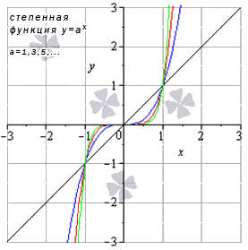
Let's analyze the power function y = x a when a is an odd positive number, for example, a = 1 , 3 , 5 …

For clarity, we indicate the graphs of such power functions: y = x (black color of the graph), y = x 3 (blue color of the chart), y = x 5 (red color of the graph), y = x 7 (green graph). When a = 1 , we get a linear function y = x .

Definition 6

Properties of a power function when the exponent is an odd positive

• the function is increasing for x ∈ (- ∞ ; + ∞) ;
• the function is convex for x ∈ (- ∞ ; 0 ] and concave for x ∈ [ 0 ; + ∞) (excluding the linear function);
• the inflection point has coordinates (0 ; 0) (excluding the linear function);
• there are no asymptotes;
• function passing points: (- 1 ; - 1) , (0 ; 0) , (1 ; 1) .

Let's analyze the power function y = x a when a is an even positive number, for example, a = 2 , 4 , 6 ...

For clarity, we indicate the graphs of such power functions: y \u003d x 2 (black color of the graph), y = x 4 (blue color of the graph), y = x 8 (red color of the graph). When a = 2, we get a quadratic function whose graph is a quadratic parabola.

Definition 7

Properties of a power function when the exponent is even positive:

• domain of definition: x ∈ (- ∞ ; + ∞) ;
• decreasing for x ∈ (- ∞ ; 0 ] ;
• the function is concave for x ∈ (- ∞ ; + ∞) ;
• there are no inflection points;
• there are no asymptotes;
• function passing points: (- 1 ; 1) , (0 ; 0) , (1 ; 1) .

The figure below shows examples of exponential function graphs y = x a when a is an odd negative number: y = x - 9 (black color of the graph); y = x - 5 (blue color of the graph); y = x - 3 (red color of the graph); y = x - 1 (green graph). When a \u003d - 1, we get an inverse proportionality, the graph of which is a hyperbola.

Definition 8

Power function properties when the exponent is odd negative:

When x \u003d 0, we get a discontinuity of the second kind, since lim x → 0 - 0 x a \u003d - ∞, lim x → 0 + 0 x a \u003d + ∞ for a \u003d - 1, - 3, - 5, .... Thus, the straight line x = 0 is a vertical asymptote;

• range: y ∈ (- ∞ ; 0) ∪ (0 ; + ∞) ;
• the function is odd because y (- x) = - y (x) ;
• the function is decreasing for x ∈ - ∞ ; 0 ∪ (0 ; + ∞) ;
• the function is convex for x ∈ (- ∞ ; 0) and concave for x ∈ (0 ; + ∞) ;
• there are no inflection points;

k = lim x → ∞ x a x = 0 , b = lim x → ∞ (x a - k x) = 0 ⇒ y = k x + b = 0 when a = - 1 , - 3 , - 5 , . . . .

• function passing points: (- 1 ; - 1) , (1 ; 1) .

The figure below shows examples of power function graphs y = x a when a is an even negative number: y = x - 8 (chart in black); y = x - 4 (blue color of the graph); y = x - 2 (red color of the graph).

Definition 9

Power function properties when the exponent is even negative:

• domain of definition: x ∈ (- ∞ ; 0) ∪ (0 ; + ∞) ;

When x \u003d 0, we get a discontinuity of the second kind, since lim x → 0 - 0 x a \u003d + ∞, lim x → 0 + 0 x a \u003d + ∞ for a \u003d - 2, - 4, - 6, .... Thus, the straight line x = 0 is a vertical asymptote;

• the function is even because y (- x) = y (x) ;
• the function is increasing for x ∈ (- ∞ ; 0) and decreasing for x ∈ 0 ; +∞ ;
• the function is concave for x ∈ (- ∞ ; 0) ∪ (0 ; + ∞) ;
• there are no inflection points;
• the horizontal asymptote is a straight line y = 0 because:

k = lim x → ∞ x a x = 0 , b = lim x → ∞ (x a - k x) = 0 ⇒ y = k x + b = 0 when a = - 2 , - 4 , - 6 , . . . .

• function passing points: (- 1 ; 1) , (1 ; 1) .

From the very beginning, pay attention to the following aspect: in the case when a is a positive fraction with an odd denominator, some authors take the interval - ∞ as the domain of definition of this power function; + ∞ , stipulating that the exponent a is an irreducible fraction. At the moment, the authors of many educational publications on algebra and the beginnings of analysis DO NOT DEFINE power functions, where the exponent is a fraction with an odd denominator for negative values ​​of the argument. Further, we will adhere to just such a position: we take the set [ 0 ; +∞) . Recommendation for students: find out the teacher's point of view at this point in order to avoid disagreements.

So let's take a look at the power function y = x a when the exponent is a rational or irrational number provided that 0< a < 1 .

Let us illustrate with graphs the power functions y = x a when a = 11 12 (chart in black); a = 5 7 (red color of the graph); a = 1 3 (blue color of the chart); a = 2 5 (green color of the graph).

Other values ​​of the exponent a (assuming 0< a < 1) дадут аналогичный вид графика.

Definition 10

Power function properties at 0< a < 1:

• range: y ∈ [ 0 ; +∞) ;
• the function is increasing for x ∈ [ 0 ; +∞) ;
• the function has convexity for x ∈ (0 ; + ∞) ;
• there are no inflection points;
• there are no asymptotes;

Let's analyze the power function y = x a when the exponent is a non-integer rational or irrational number provided that a > 1 .

We illustrate the graphs of the power function y \u003d x a under given conditions using the following functions as an example: y \u003d x 5 4, y \u003d x 4 3, y \u003d x 7 3, y \u003d x 3 π (black, red, blue, green graphs, respectively).

Other values ​​of the exponent a under the condition a > 1 will give a similar view of the graph.

Definition 11

Power function properties for a > 1:

• domain of definition: x ∈ [ 0 ; +∞) ;
• range: y ∈ [ 0 ; +∞) ;
• this function is a function of general form (it is neither odd nor even);
• the function is increasing for x ∈ [ 0 ; +∞) ;
• the function is concave for x ∈ (0 ; + ∞) (when 1< a < 2) и выпуклость при x ∈ [ 0 ; + ∞) (когда a > 2);
• there are no inflection points;
• there are no asymptotes;
• function passing points: (0 ; 0) , (1 ; 1) .

We draw your attention! When a is a negative fraction with an odd denominator, in the works of some authors there is a view that the domain of definition in this case is the interval - ∞; 0 ∪ (0 ; + ∞) with the proviso that the exponent a is an irreducible fraction. At the moment, the authors of educational materials on algebra and the beginnings of analysis DO NOT DEFINE power functions with an exponent in the form of a fraction with an odd denominator for negative values ​​of the argument. Further, we adhere to just such a view: we take the set (0 ; + ∞) as the domain of power functions with fractional negative exponents. Suggestion for students: Clarify your teacher's vision at this point to avoid disagreement.

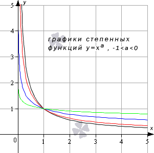
We continue the topic and analyze the power function y = x a provided: - 1< a < 0 .

Here is a drawing of graphs of the following functions: y = x - 5 6 , y = x - 2 3 , y = x - 1 2 2 , y = x - 1 7 (black, red, blue, green lines, respectively).

Definition 12

Power function properties at - 1< a < 0:

lim x → 0 + 0 x a = + ∞ when - 1< a < 0 , т.е. х = 0 – вертикальная асимптота;

• range: y ∈ 0 ; +∞ ;
• this function is a function of general form (it is neither odd nor even);
• there are no inflection points;

The drawing below shows graphs of power functions y = x - 5 4 , y = x - 5 3 , y = x - 6 , y = x - 24 7 (black, red, blue, green colors of the curves, respectively).

Definition 13

Power function properties for a< - 1:

• domain of definition: x ∈ 0 ; +∞ ;

lim x → 0 + 0 x a = + ∞ when a< - 1 , т.е. х = 0 – вертикальная асимптота;

• range: y ∈ (0 ; + ∞) ;
• this function is a function of general form (it is neither odd nor even);
• the function is decreasing for x ∈ 0; +∞ ;
• the function is concave for x ∈ 0; +∞ ;
• there are no inflection points;
• horizontal asymptote - straight line y = 0 ;
• function passing point: (1 ; 1) .

When a \u003d 0 and x ≠ 0, we get the function y \u003d x 0 \u003d 1, which determines the line from which the point (0; 1) is excluded (we agreed that the expression 0 0 will not be given any value).

The exponential function has the form y = a x , where a > 0 and a ≠ 1 , and the graph of this function looks different based on the value of the base a . Let's consider special cases.

First, let's analyze the situation when the base of the exponential function has a value from zero to one (0< a < 1) . An illustrative example is the graphs of functions for a = 1 2 (blue color of the curve) and a = 5 6 (red color of the curve).

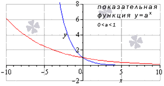
The graphs of the exponential function will have a similar form for other values ​​​​of the base, provided that 0< a < 1 .

Definition 14

Properties of an exponential function when the base is less than one:

• range: y ∈ (0 ; + ∞) ;
• this function is a function of general form (it is neither odd nor even);
• an exponential function whose base is less than one is decreasing over the entire domain of definition;
• there are no inflection points;
• the horizontal asymptote is the straight line y = 0 with the variable x tending to + ∞ ;

Now consider the case when the base of the exponential function is greater than one (a > 1).

Let's illustrate this special case with the graph of exponential functions y = 3 2 x (blue color of the curve) and y = e x (red color of the graph).

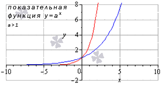
Other values ​​​​of the base, greater than one, will give a similar view of the graph of the exponential function.

Definition 15

Properties of the exponential function when the base is greater than one:

• the domain of definition is the entire set of real numbers;
• range: y ∈ (0 ; + ∞) ;
• this function is a function of general form (it is neither odd nor even);
• an exponential function whose base is greater than one is increasing for x ∈ - ∞ ; +∞ ;
• the function is concave for x ∈ - ∞ ; +∞ ;
• there are no inflection points;
• horizontal asymptote - straight line y = 0 with variable x tending to - ∞ ;
• function passing point: (0 ; 1) .

The logarithmic function has the form y = log a (x) , where a > 0 , a ≠ 1 .

Such a function is defined only for positive values ​​of the argument: for x ∈ 0 ; +∞ .

The graph of the logarithmic function has a different form, based on the value of the base a.

Consider first the situation when 0< a < 1 . Продемонстрируем этот частный случай графиком логарифмической функции при a = 1 2 (синий цвет кривой) и а = 5 6 (красный цвет кривой).

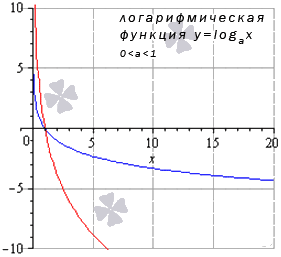
Other values ​​of the base, not greater than one, will give a similar view of the graph.

Definition 16

Properties of a logarithmic function when the base is less than one:

• domain of definition: x ∈ 0 ; +∞ . As x tends to zero from the right, the values ​​of the function tend to + ∞;
• range: y ∈ - ∞ ; +∞ ;
• this function is a function of general form (it is neither odd nor even);
• logarithmic
• the function is concave for x ∈ 0; +∞ ;
• there are no inflection points;
• there are no asymptotes;

Now let's analyze a special case when the base of the logarithmic function is greater than one: a > 1 . In the drawing below, there are graphs of logarithmic functions y = log 3 2 x and y = ln x (blue and red colors of the graphs, respectively).

Other values ​​of the base greater than one will give a similar view of the graph.

Definition 17

Properties of a logarithmic function when the base is greater than one:

• domain of definition: x ∈ 0 ; +∞ . As x tends to zero from the right, the values ​​of the function tend to - ∞;
• range: y ∈ - ∞ ; + ∞ (the whole set of real numbers);
• this function is a function of general form (it is neither odd nor even);
• the logarithmic function is increasing for x ∈ 0; +∞ ;
• the function has convexity for x ∈ 0; +∞ ;
• there are no inflection points;
• there are no asymptotes;
• function passing point: (1 ; 0) .

Trigonometric functions are sine, cosine, tangent and cotangent. Let's analyze the properties of each of them and the corresponding graphs.

In general, all trigonometric functions are characterized by the property of periodicity, i.e. when the values ​​of the functions are repeated for different values ​​of the argument that differ from each other by the value of the period f (x + T) = f (x) (T is the period). Thus, the item "least positive period" is added to the list of properties of trigonometric functions. In addition, we will indicate such values ​​of the argument for which the corresponding function vanishes.

1. Sine function: y = sin(x)

The graph of this function is called a sine wave.

Definition 18

Properties of the sine function:

• domain of definition: the whole set of real numbers x ∈ - ∞ ; +∞ ;
• the function vanishes when x = π k , where k ∈ Z (Z is the set of integers);
• the function is increasing for x ∈ - π 2 + 2 π · k ; π 2 + 2 π k , k ∈ Z and decreasing for x ∈ π 2 + 2 π k ; 3 π 2 + 2 π k , k ∈ Z ;
• the sine function has local maxima at the points π 2 + 2 π · k ; 1 and local minima at points - π 2 + 2 π · k ; - 1 , k ∈ Z ;
• the sine function is concave when x ∈ - π + 2 π k; 2 π k , k ∈ Z and convex when x ∈ 2 π k ; π + 2 π k , k ∈ Z ;
• there are no asymptotes.

1. cosine function: y=cos(x)

The graph of this function is called a cosine wave.

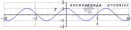
Definition 19

Properties of the cosine function:

• domain of definition: x ∈ - ∞ ; +∞ ;
• the smallest positive period: T \u003d 2 π;
• range: y ∈ - 1 ; one ;
• this function is even, since y (- x) = y (x) ;
• the function is increasing for x ∈ - π + 2 π · k ; 2 π · k , k ∈ Z and decreasing for x ∈ 2 π · k ; π + 2 π k , k ∈ Z ;
• the cosine function has local maxima at points 2 π · k ; 1 , k ∈ Z and local minima at the points π + 2 π · k ; - 1 , k ∈ z ;
• the cosine function is concave when x ∈ π 2 + 2 π · k ; 3 π 2 + 2 π k , k ∈ Z and convex when x ∈ - π 2 + 2 π k ; π 2 + 2 π · k , k ∈ Z ;
• inflection points have coordinates π 2 + π · k ; 0 , k ∈ Z
• there are no asymptotes.

1. Tangent function: y = t g (x)

The graph of this function is called tangentoid.

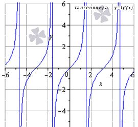
Definition 20

Properties of the tangent function:

• domain of definition: x ∈ - π 2 + π · k ; π 2 + π k , where k ∈ Z (Z is the set of integers);
• The behavior of the tangent function on the boundary of the domain of definition lim x → π 2 + π · k + 0 t g (x) = - ∞ , lim x → π 2 + π · k - 0 t g (x) = + ∞ . Thus, the lines x = π 2 + π · k k ∈ Z are vertical asymptotes;
• the function vanishes when x = π k for k ∈ Z (Z is the set of integers);
• range: y ∈ - ∞ ; +∞ ;
• this function is odd because y (- x) = - y (x) ;
• the function is increasing at - π 2 + π · k ; π 2 + π k , k ∈ Z ;
• the tangent function is concave for x ∈ [ π · k ; π 2 + π k) , k ∈ Z and convex for x ∈ (- π 2 + π k ; π k ] , k ∈ Z ;
• inflection points have coordinates π k; 0 , k ∈ Z ;

1. Cotangent function: y = c t g (x)

The graph of this function is called the cotangentoid. .

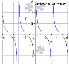
Definition 21

Properties of the cotangent function:

• domain of definition: x ∈ (π k ; π + π k) , where k ∈ Z (Z is the set of integers);

Behavior of the cotangent function on the boundary of the domain of definition lim x → π · k + 0 t g (x) = + ∞ , lim x → π · k - 0 t g (x) = - ∞ . Thus, the lines x = π k k ∈ Z are vertical asymptotes;

• the smallest positive period: T \u003d π;
• the function vanishes when x = π 2 + π k for k ∈ Z (Z is the set of integers);
• range: y ∈ - ∞ ; +∞ ;
• this function is odd because y (- x) = - y (x) ;
• the function is decreasing for x ∈ π · k ; π + π k , k ∈ Z ;
• the cotangent function is concave for x ∈ (π k ; π 2 + π k ] , k ∈ Z and convex for x ∈ [ - π 2 + π k ; π k) , k ∈ Z ;
• inflection points have coordinates π 2 + π · k ; 0 , k ∈ Z ;
• there are no oblique and horizontal asymptotes.

The inverse trigonometric functions are the arcsine, arccosine, arctangent, and arccotangent. Often, due to the presence of the prefix "arc" in the name, inverse trigonometric functions are called arc functions. .

1. Arcsine function: y = a r c sin (x)

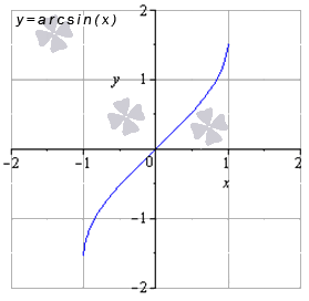
Definition 22

Properties of the arcsine function:

• this function is odd because y (- x) = - y (x) ;
• the arcsine function is concave for x ∈ 0; 1 and convexity for x ∈ - 1 ; 0;
• inflection points have coordinates (0 ; 0) , it is also the zero of the function;
• there are no asymptotes.

1. Arccosine function: y = a r c cos (x)

Definition 23

Arccosine function properties:

• domain of definition: x ∈ - 1 ; one ;
• range: y ∈ 0 ; π;
• this function is of general form (neither even nor odd);
• the function is decreasing on the entire domain of definition;
• the arccosine function is concave for x ∈ - 1 ; 0 and convexity for x ∈ 0 ; one ;
• inflection points have coordinates 0 ; π2;
• there are no asymptotes.

1. Arctangent function: y = a r c t g (x)

Definition 24

Arctangent function properties:

• domain of definition: x ∈ - ∞ ; +∞ ;
• range: y ∈ - π 2 ; π2;
• this function is odd because y (- x) = - y (x) ;
• the function is increasing over the entire domain of definition;
• the arctangent function is concave for x ∈ (- ∞ ; 0 ] and convex for x ∈ [ 0 ; + ∞) ;
• the inflection point has coordinates (0; 0), it is also the zero of the function;
• horizontal asymptotes are straight lines y = - π 2 for x → - ∞ and y = π 2 for x → + ∞ (the asymptotes in the figure are green lines).

1. Arc cotangent function: y = a r c c t g (x)

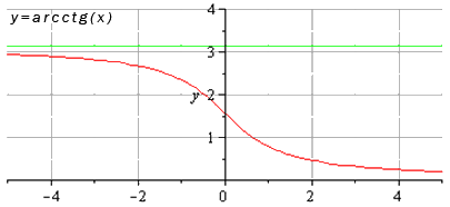
Definition 25

Arc cotangent function properties:

• domain of definition: x ∈ - ∞ ; +∞ ;
• range: y ∈ (0 ; π) ;
• this function is of a general type;
• the function is decreasing on the entire domain of definition;
• the arc cotangent function is concave for x ∈ [ 0 ; + ∞) and convexity for x ∈ (- ∞ ; 0 ] ;
• the inflection point has coordinates 0 ; π2;
• horizontal asymptotes are straight lines y = π at x → - ∞ (green line in the drawing) and y = 0 at x → + ∞.

If you notice a mistake in the text, please highlight it and press Ctrl+Enter

Once you really understand what a function is (you may have to read the lesson more than once), you will be able to solve problems with functions with more confidence.

In this lesson, we will analyze how to solve the main types of function problems and function graphs.

How to get the value of a function

Let's consider the task. The function is given by the formula " y \u003d 2x - 1"

1. Calculate " y"When" x \u003d 15 "
2. Find the value " x", At which the value " y "is equal to" −19 ".

In order to calculate " y"With" x \u003d 15"It is enough to substitute the required numerical value into the function instead of" x".

The solution entry looks like this:

y(15) = 2 15 - 1 = 30 - 1 = 29

In order to find " x"According to the known" y", It is necessary to substitute a numerical value instead of" y "in the function formula.

That is, now, on the contrary, to search for " x"We substitute in the function" y \u003d 2x - 1 "Instead of" y ", the number" −19".

−19 = 2x − 1

We have obtained a linear equation with an unknown "x", which is solved according to the rules for solving linear equations.

Remember!

Don't forget about the transfer rule in equations.

When transferring from the left side of the equation to the right (and vice versa), the letter or number changes sign to opposite.

−19 = 2x − 1
0 = 2x − 1 + 19
-2x = -1 + 19
−2x = 18

As with solving a linear equation, to find the unknown, now we need to multiply both left and right side to "−1" to change the sign.

-2x = 18 | (−1)
2x = −18

Now let's divide both the left and right sides by "2" to find "x".

2x = 18 | (:2)
x=9

How to check if equality is true for a function

Let's consider the task. The function is given by the formula "f(x) = 2 − 5x".

Is the equality "f(−2) = −18" true?

To check whether the equality is true, you need to substitute the numerical value “x = −2" into the function " f (x) \u003d 2 - 5x"And compare with what happens in the calculations.

Important!

When you substitute a negative number for "x", be sure to enclose it in brackets.

Not right

Correctly

With the help of calculations, we got "f(−2) = 12".

This means that "f(−2) = −18" for the function "f(x) = 2 − 5x" is not a valid equality.

How to check if a point belongs to a graph of a function

Consider the function " y \u003d x 2 −5x + 6"

It is required to find out whether the point with coordinates (1; 2) belongs to the graph of this function.

For this task, there is no need to plot a given function.

Remember!

To determine whether a point belongs to a function, it is enough to substitute its coordinates into the function (coordinate along the axis "Ox" instead of "x" and the coordinate along the axis "Oy" instead of "y").

If this works out true equality, so the point belongs to the function.

Let's return to our task. Substitute in the function "y \u003d x 2 - 5x + 6" the coordinates of the point (1; 2).

Instead of " x"We substitute" 1". Instead of " y"Substitute" 2».

2 = 1 2 − 5 1 + 6
2 = 1 − 5 + 6
2 = −4 + 6
2 = 2 (correct)

We have obtained the correct equality, which means that the point with coordinates (1; 2) belongs to the given function.

Now let's check the point with coordinates (0; 1) . Does she belong
functions "y \u003d x 2 - 5x + 6"?

Instead of "x", let's substitute "0". Instead of " y"Substitute" 1».

1 = 0 2 − 5 0 + 6
1 = 0 − 0 + 6
1 = 6 (wrong)

In this case, we did not get the correct equality. This means that the point with coordinates (0; 1) does not belong to the function " y \u003d x 2 - 5x + 6 "

How to get function point coordinates

From any function graph, you can take the coordinates of a point. Then you need to make sure that when substituting the coordinates in the function formula, the correct equality is obtained.

Consider the function "y(x) = −2x + 1". We have already built its schedule in the previous lesson.

Let's find on the graph of the function " y (x) \u003d -2x + 1", which is equal to" y"For x \u003d 2.

To do this, from the value " 2"On the axis" Ox", Draw a perpendicular to the graph of the function. From the point of intersection of the perpendicular and the graph of the function, draw another perpendicular to the axis "Oy".

The resulting value " −3"On the axis" Oy"And will be the desired value" y».

Let's make sure that we correctly took the coordinates of the point for x = 2
in the function "y(x) = −2x + 1".

To do this, we substitute x \u003d 2 into the formula of the function "y (x) \u003d -2x + 1". If we draw the perpendicular correctly, we should also end up with y = −3 .

y(2) = -2 2 + 1 = -4 + 1 = -3

When calculating, we also got y = −3.

This means that we correctly received the coordinates from the graph of the function.

Important!

Be sure to check all the coordinates of the point from the function graph by substituting the values ​​\u200b\u200bof "x" into the function.

When substituting the numeric value "x" into the function, the result should be the same value" y", which you got on the chart.

When obtaining the coordinates of points from the graph of the function, it is highly likely that you will make a mistake, because drawing a perpendicular to the axes is performed "by eye".

Only substituting values ​​into a function formula gives accurate results.